When at critical point, (θ − θ′)Tg = 0,
telling the properties of critical
points.
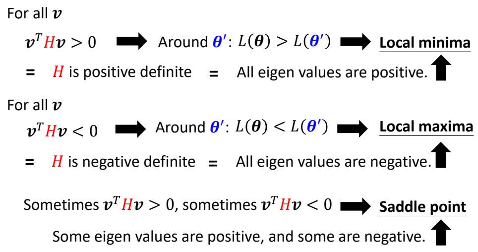
Set θ − θ′ = v:
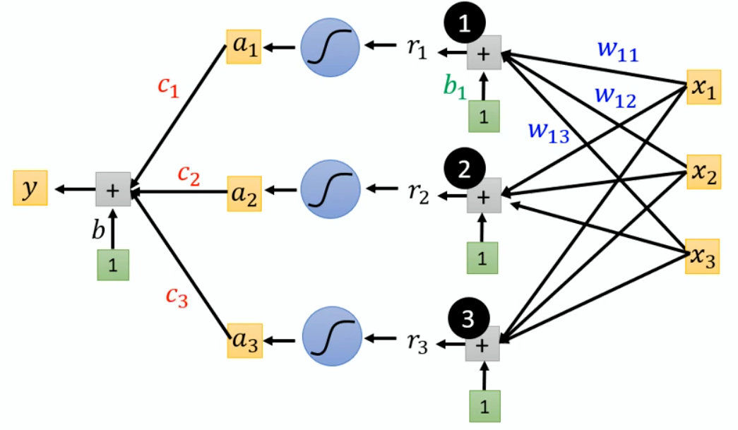
H may tell us
parameter update direction!
While u is an eigen vector
of H, λ is the eigen value of u, uTHu = uT(λu) = λ∥u∥2
Example: if u < 0, then
H < 0, then L(θ) < L(θ′)
, θ = θ′ + u,
L can be decreased.
We can escape the saddle point and decrease the loss. However,
this method is seldom used in practice.
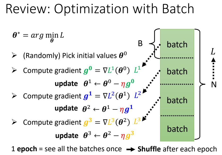
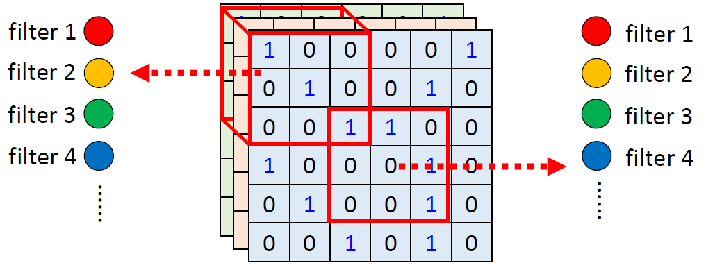
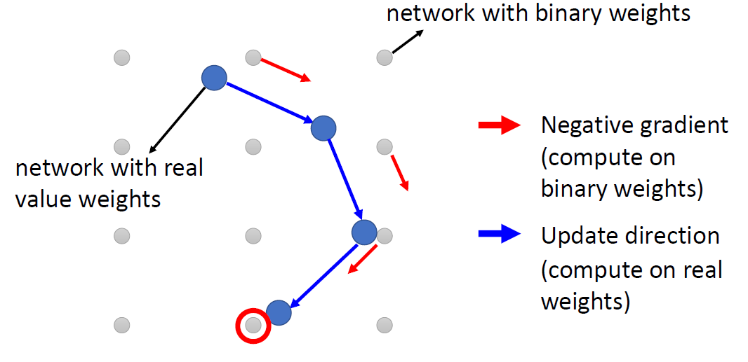
Batch & Momentum
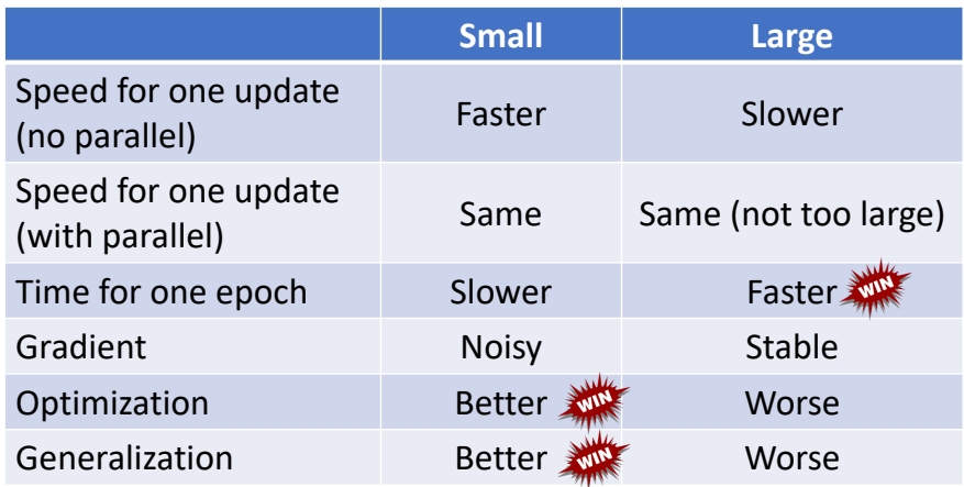
Small Batch v.s. Large Batch
Larger batch size does not require longer time to
compute gradient (unless batch size is too large)
Smaller batch requires longer time for one epoch
(longer time for seeing all data once)
Smaller batch size has better performance in optimization
“Noisy” update is better for training
Batch size is a hyperparameter you have to decide.
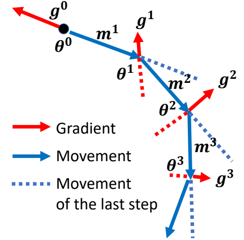
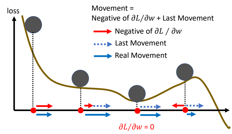
Gradient Descent + Momentum
Movement: movement of last step minus
gradient at present
Movement not just based on gradient, but previous movement.
Example:
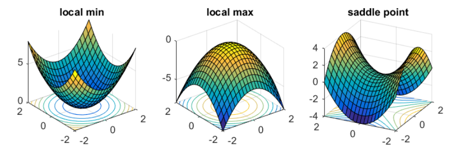
Summary
Critical points have zero gradients.
Critical points can be either saddle points or local minima.
Can be determined by the Hessian matrix.
Local minima may be rare.
It is possible to escape saddle points along the direction of eigen
vectors of the Hessian matrix.
Smaller batch size and momentum help escape critical
points.
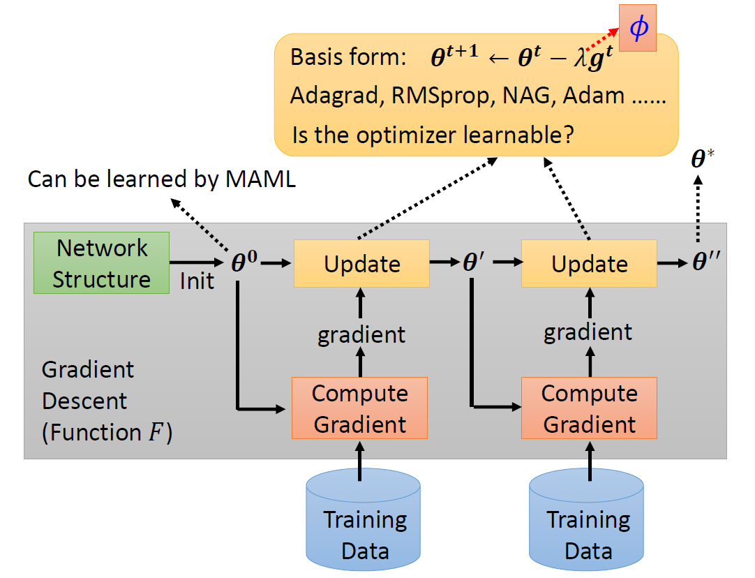
Adaptive Learning Rate
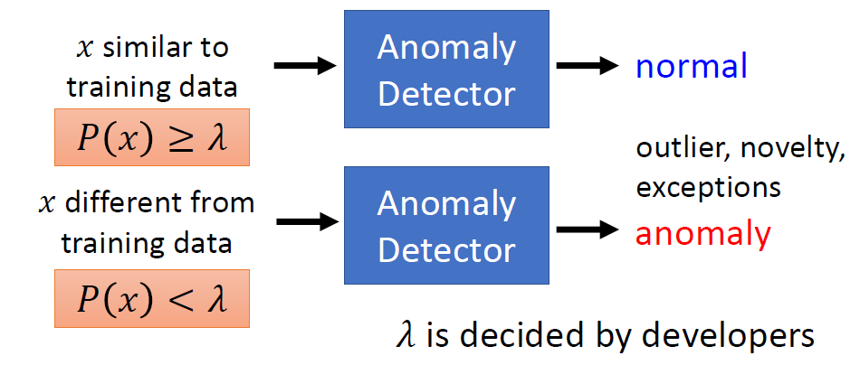
People believe training stuck because the parameters are around a
critical point, but sometimes learning rate may be the reason.
While learning rate cannot be one-size-fits-all, so
different parameters need different learning rate.
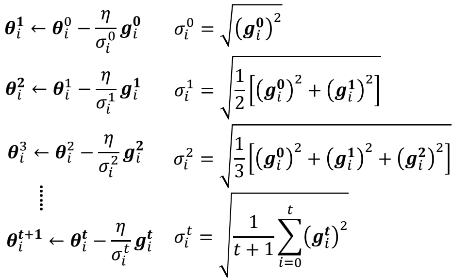
Consider update one parameter(t means iteration time, i means the ith
parameter):
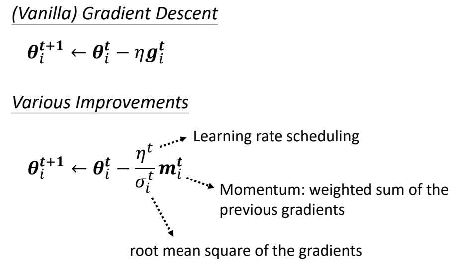
θit + 1 ← θit − ηgit
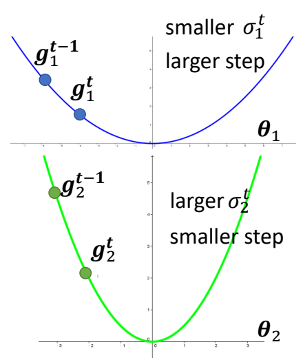
While larger gradient needs smaller learning rate and smaller
gradient needs larger learning rate, so learning rate has to be
parameter dependent:
Root Mean Square
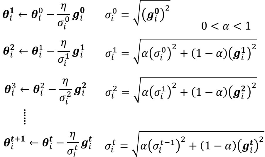
RMSProp
The recent gradient has larger influence, and the past gradients have
less influence.
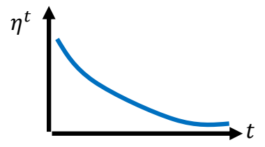
Learning Rate Scheduling
Learning Rate Decay
After the training goes, we are close to the destination, so we
reduce the learning rate.
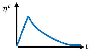
Warm Up
Increase and then decrease.
At the beginning, the estimate of σit
has large variance.
Summary of Optimization
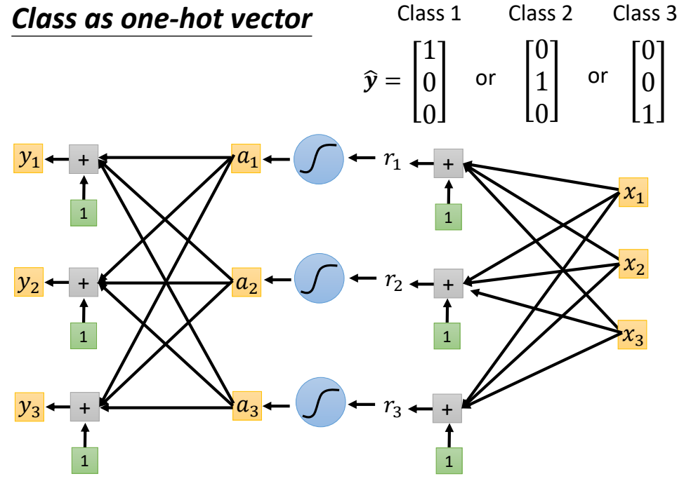
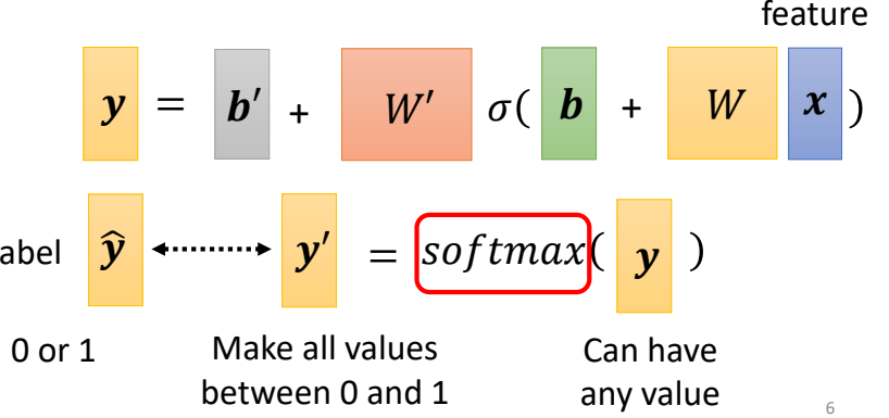
Classification
Classification as Regression
Softmax:
1 > yi′ > 0
∑iyi′ = 1
The core function of Softmax is to normalize a
model’s raw prediction scores (Logits) into a valid, interpretable
probability distribution (all probabilities >=0 and
sum=1), explicitly representing the model’s prediction confidence across
multiple mutually exclusive classes.
Loss of Classification
Mean Square Error(MSE): e = ∑i(ŷi − yi′)2
Cross-entropy: e = −∑iŷilnyi′(More Competitive)
Minimizing cross-entropy is equivalent to
maximizing likelihood.
Changing the loss function can change the difficulty of
optimization.
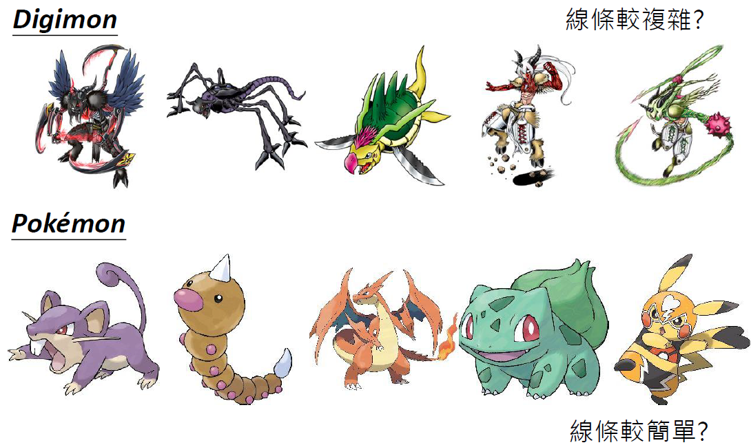
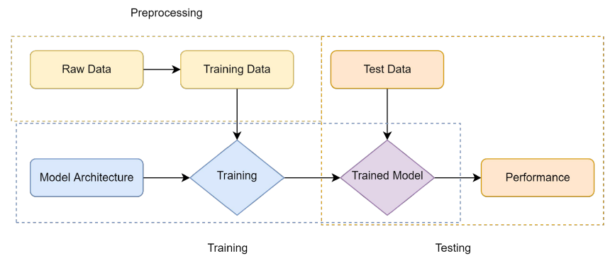
Case Study: Pokémon v.s.
Digimon
We want to find a function to classify Pokémon/Digimon
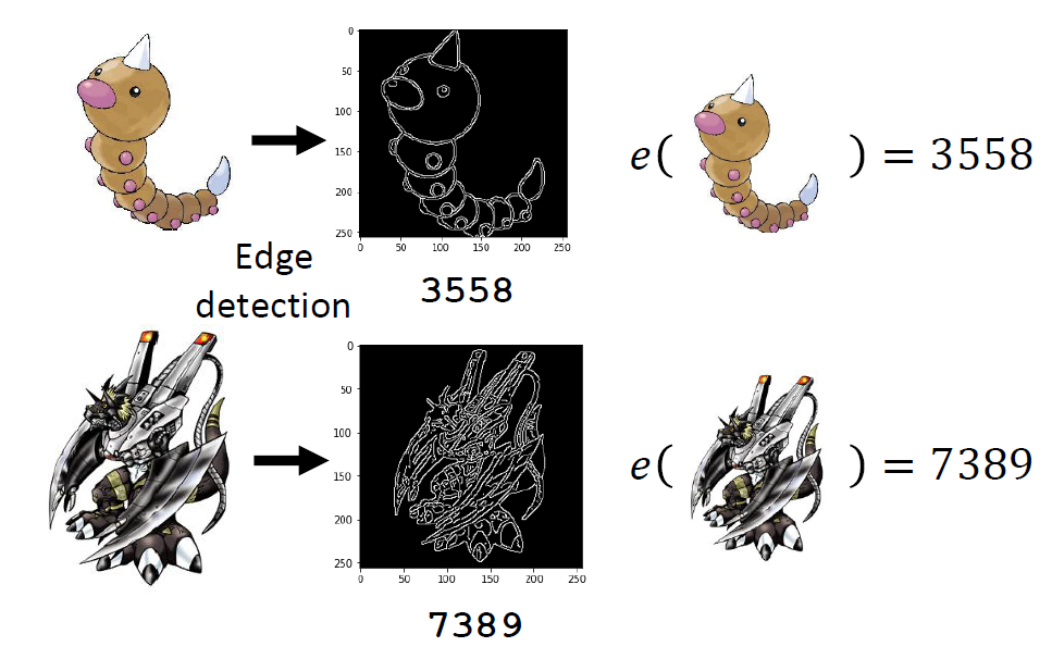
Determine a function with unknown parameters(based on domain
knowledge)
Observation
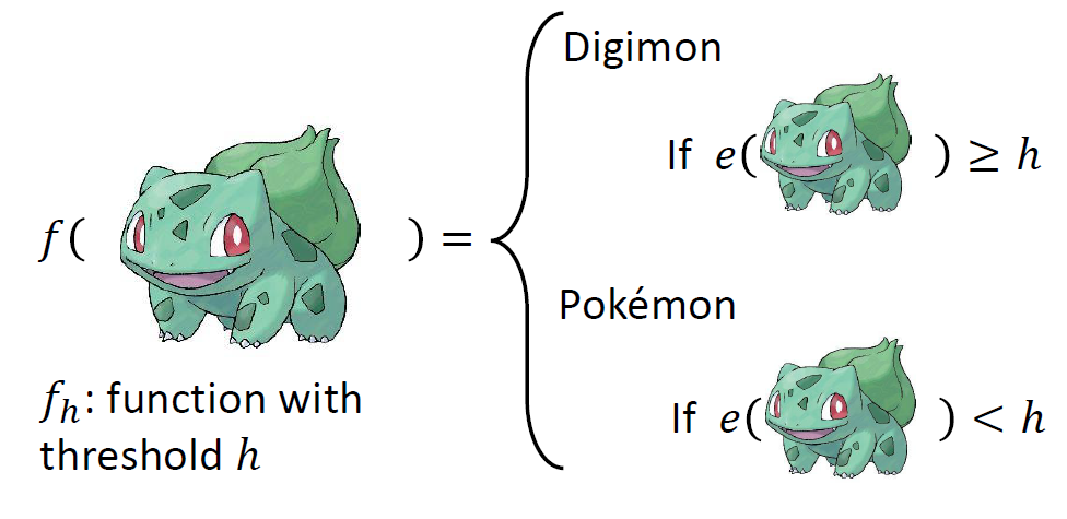
Function with Unknown
Parameters
ℋ = {1, 2, ..., 10000}, |ℋ|: model “complexity”
Loss of a function (given
data)
Given a dataset 𝒟
𝒟 = {(x1, ŷ1), (x2, ŷ2), ..., (xN, ŷN)}
Loss of a threshold h
given data set 𝒟
Error rate:
l(h, xn, ŷn)
means I(fh(xn) ≠ ŷn):
if fh(xn) ≠ ŷn,
output 1, otherwise output 0.
Of course can choose cross entropy instead.
Training Examples
If we can collect all Pokémons and Digimons in the universe 𝒟all,
we can find the best threshold hall
𝒟𝓉𝓇𝒶𝒾𝓃 is independently
and identically distributed ( i.i.d.)
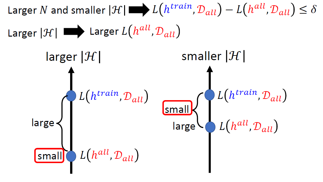
We hope L(htrain, 𝒟all)
and L(hall, 𝒟all)
are close.
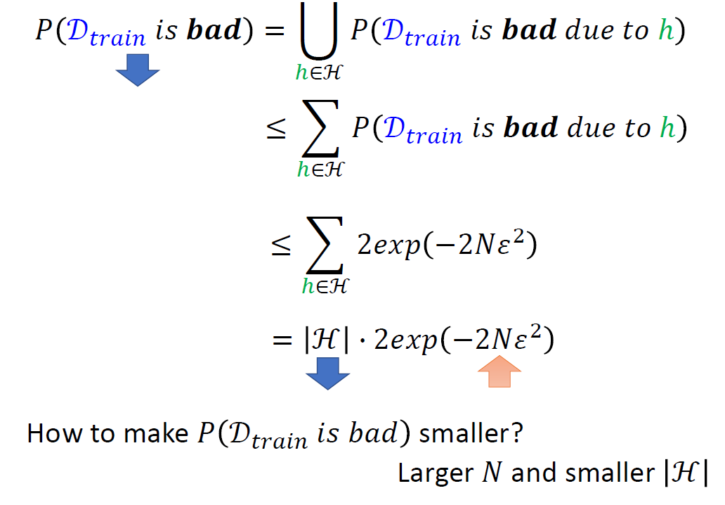
We want L(htrain, 𝒟all) − L(hall, 𝒟all) ≤ δ
So 𝒟train
has to fulfill: ∀h ∈ ℋ, |L(h, 𝒟train) − L(h, 𝒟all)| ≤ ϵ,
ϵ = δ/2
Probability of Failure
The following discussion is model-agnostic.
In the following discussion, we don’t have assumption about
data distribution.
In the following discussion, we can use any loss
function.
Each point is a training set.
image-20250531143321759
Hoeffding’s Inequality:
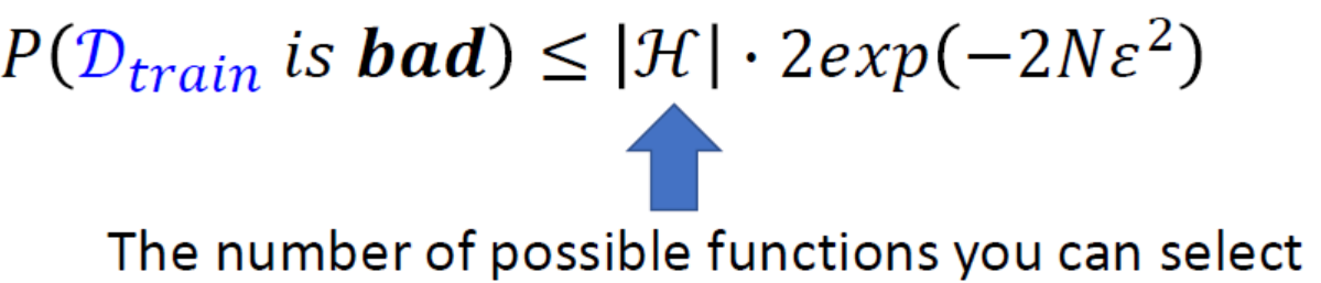
Model Complexity
What if the parameters are continuous?
Answer 1 : Everything that happens in a computer is
discrete.
Answer 2 : VC dimension
Why don’t we simply use a very small |ℋ| ?
smaller |ℋ| means fewer candidates
in h ∈ ℋ
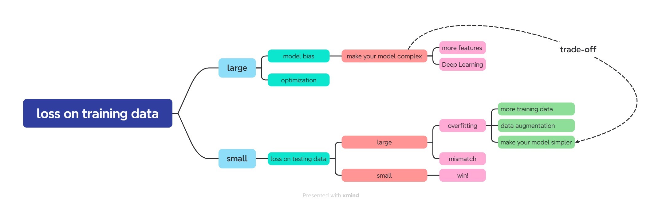
Tradeoff of Model Complexity
How to find best balance? DEEP LEARNING.
Homework 2:
Framewise phoneme prediction from speech
Data Preprocessing: Extract MFCC features from raw waveform
Classification: Perform framewise phoneme classification using
pre-extracted MFCC features
Report Questions
Implement 2 models with approximately the same number of parameters,
(A) one narrower and deeper (e.g. hidden_layers=6, hidden_dim=1024) and
(B) the other wider and shallower (e.g. hidden_layers=2,
hidden_dim=1700). Report training/validation accuracies for both
models.
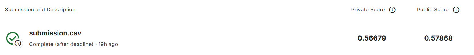
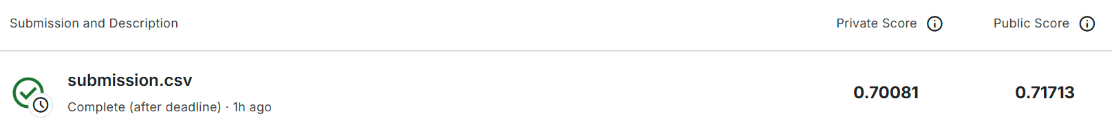
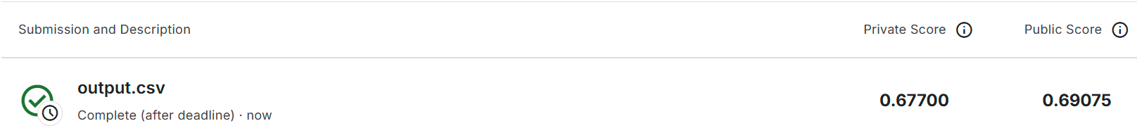
hidden_layers=6, hidden_dim=1024: acc 0.47458
hidden_layers=2, hidden_dim=1700: acc 0.47491
Add dropout layers, and report training/validation accuracies with
dropout rates equal to (A) 0.25/(B) 0.5/(C) 0.75 respectively.
# Normally, We don't need augmentations in testing and validation.
# All we need here is to resize the PIL image and transform it into Tensor.
test_tfm = transforms.Compose([
    transforms.Resize((128, 128)),
    transforms.ToTensor(),
])

# However, it is also possible to use augmentation in the testing phase.
# You may use train_tfm to produce a variety of images and then test using ensemble methods
train_tfm = transforms.Compose([
    # Resize the image into a fixed shape (height = width = 128)
    transforms.Resize((128, 128)),
    # You may add some transforms here.
    # 95%概率做随机增强(TrivialAugmentWide),10%概率保持原图.
    transforms.RandomChoice(transforms=[
        # Apply TrivialAugmentWide data augmentation method
        transforms.TrivialAugmentWide(),

        # Return original image
        transforms.Lambda(lambda x: x),
    ],
                            p=[0.95, 0.05]),
    # ToTensor() should be the last one of the transforms.
    transforms.ToTensor(),
])
Configuration
1
2
3
4
5
# The number of training epochs and patience. n_epochs = 20 patience = 10# If no improvement in 'patience' epochs, early stop
# Initialize optimizer, you may fine-tune some hyperparameters such as learning rate on your own.
optimizer = torch.optim.Adam(model.parameters(), lr=3e-4, weight_decay=1e-5)
scheduler = torch.optim.lr_scheduler.ReduceLROnPlateau(optimizer, mode='max', factor=0.8, patience=patience/2,threshold=0.05)
# 在每个epoch验证后加上
scheduler.step(best_acc)
classClassifier(nn.Module): def__init__(self, d_model=512, n_spks=600, dropout=0.2): super().__init__() # Project the dimension of features from that of input into d_model. self.prenet = nn.Linear(40, d_model) # TODO: # Change Transformer to Conformer. # https://arxiv.org/abs/2005.08100 self.encoder_layer = nn.TransformerEncoderLayer( d_model=d_model, dim_feedforward=256, nhead=32 ) self.encoder = nn.TransformerEncoder(self.encoder_layer, num_layers=2)
# Project the the dimension of features from d_model into speaker nums. self.pred_layer = nn.Sequential( nn.Linear(d_model, 2 * d_model), nn.ReLU(), nn.Dropout(dropout), nn.Linear(2 * d_model, n_spks), )
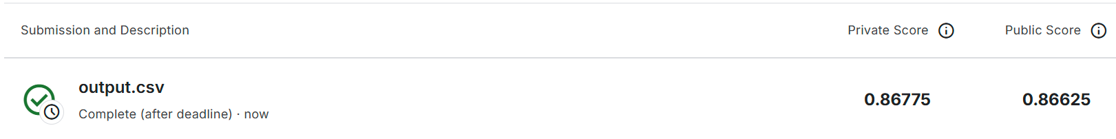
Output:
image-20250605154149324
Strong Baseline
Construct Conformer, which is a variety of
Transformer.
defget_rate(d_model, step_num, warmup_step): # TODO: Change lr from constant to the equation shown above lr = 1.0 / math.sqrt(d_model) * min(1.0 / math.sqrt(step_num), step_num / (warmup_step * math.sqrt(warmup_step))) return lr
# cpu threads when fetching & processing data. num_workers=2, # batch size in terms of tokens. gradient accumulation increases the effective batchsize. max_tokens=8192, accum_steps=2,
# the lr s calculated from Noam lr scheduler. you can tune the maximum lr by this factor. lr_factor=2., lr_warmup=4000,
# maximum epochs for training (Medium) max_epoch=30, start_epoch=1,
# beam size for beam search beam=5, # generate sequences of maximum length ax + b, where x is the source length max_len_a=1.2, max_len_b=10, # when decoding, post process sentence by removing sentencepiece symbols and jieba tokenization. post_process = "sentencepiece",
# checkpoints keep_last_epochs=5, resume=None, # if resume from checkpoint name (under config.savedir)
defbuild_model(args, task): """ build a model instance based on hyperparameters """ src_dict, tgt_dict = task.source_dictionary, task.target_dictionary
# patches on default parameters for Transformer (those not set above) from fairseq.models.transformer import base_architecture base_architecture(arch_args)
add_transformer_args(arch_args)
Boss Baseline
Apply back-translation
Train a backward model by switching languages
image-20250608152524850
Translate monolingual data with backward model to obtain
synthetic data
Complete TODOs in the sample code
All the TODOs can be completed by using commands from earlier
cells
Train a stronger forward model with the new data
If done correctly, 30 epochs on new data should pass the
baseline
Configuration for
experiments
Set BACK_TRANSLATION to True in
the configuration for experiments and run. Train a
back-translation model and process the corresponding corpus.
Set BACK_TRANSLATION to False in
the configuration for experiments and run. Train with
the corpus of ted2020 and mono (back-translation).
defbuild_model(args, task): """ build a model instance based on hyperparameters """ src_dict, tgt_dict = task.source_dictionary, task.target_dictionary
# patches on default parameters for Transformer (those not set above) from fairseq.models.transformer import base_architecture base_architecture(arch_args)
add_transformer_args(arch_args)
Back-translation
TODO: clean corpus
remove sentences that are too long or too short
unify punctuation
hint: you can use clean_s() defined above to do this
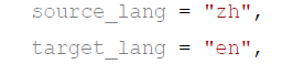
defclean_mono_corpus(prefix, l, ratio=9, max_len=1000, min_len=1): if Path(f'{prefix}.clean.zh').exists(): print(f'{prefix}.clean.zh exists. skipping clean.') return withopen(f'{prefix}', 'r') as l_in_f: withopen(f'{prefix}.clean.zh', 'w') as l_out_f: for s in l_in_f: s = s.strip() s = clean_s(s, l) s_len = len_s(s, l) if min_len > 0: # remove short sentence if s_len < min_len: continue if max_len > 0: # remove long sentence if s_len > max_len: continue print(s, file=l_out_f)
for lang in [src_lang, tgt_lang]: out_path = mono_prefix / f'mono.tok.{lang}' if out_path.exists(): print(f"{out_path} exists. skipping spm_encode.") else: withopen(out_path, 'w') as out_f: withopen(f'{in_path}.{lang}', 'r') as in_f: for line in in_f: line = line.strip() tok = spm_model.encode(line, out_type=str) print(' '.join(tok), file=out_f)
TODO: Generate
synthetic data with backward model
Add binarized monolingual data to the original data directory, and
name it with “split_name”
# Combine prediction_file (.en) and mono.zh (.zh) into a new dataset.
#
# hint: tokenize prediction_file with the spm model
!cp ./prediction.txt {mono_prefix}/'ted_zh_corpus.deduped.clean.en'
spm_encode(prefix, vocab_size, mono_prefix)
# spm_model.encode(line, out_type=str)
# output: ./DATA/rawdata/mono/mono.tok.en & mono.tok.zh
#
# hint: use fairseq to binarize these two files again
binpath = Path('./DATA/data-bin/synthetic')
src_dict_file = './DATA/data-bin/ted2020/dict.en.txt'
tgt_dict_file = src_dict_file
monopref = ./DATA/rawdata/mono/mono.tok # or whatever path after applying subword tokenization, w/o the suffix (.zh/.en)
if binpath.exists():
     print(binpath, "exists, will not overwrite!")
else:
     !python -m fairseq_cli.preprocess\
         	--source-lang 'zh'\
         	--target-lang 'en'\
         	--trainpref {monopref}\
	        --destdir {binpath}\
	        --srcdict {src_dict_file}\
            --tgtdict {tgt_dict_file}\
	        --workers 2
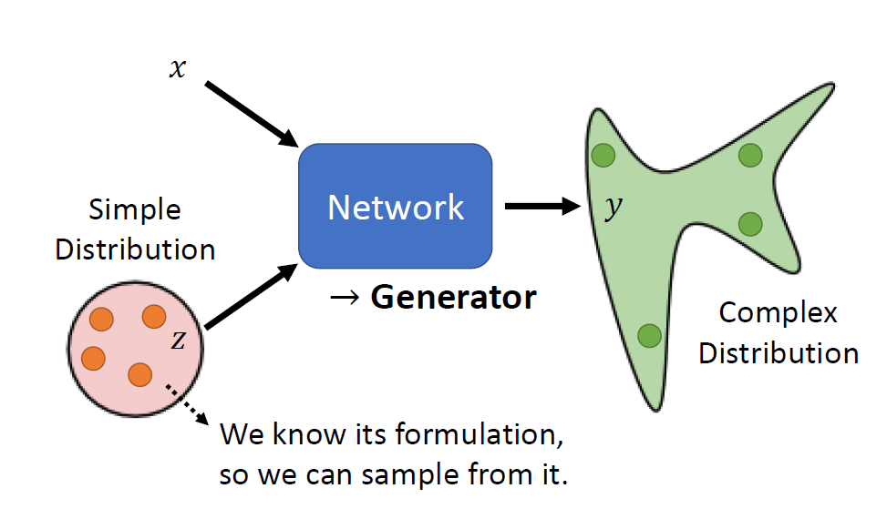
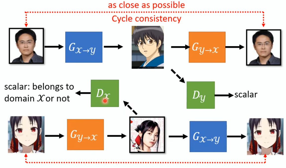
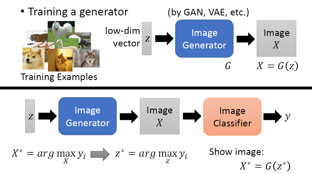
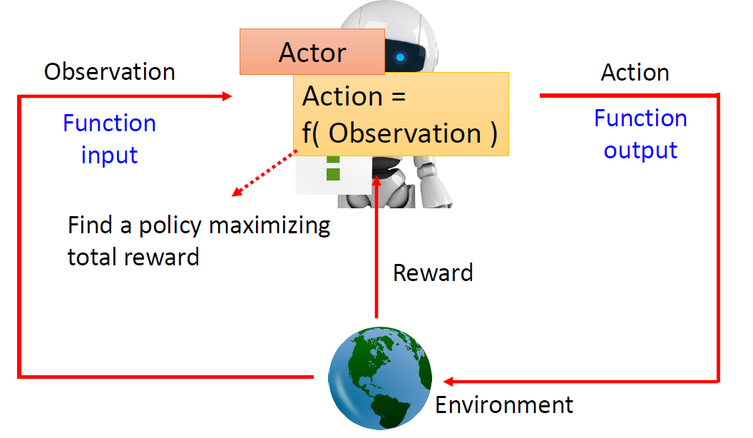
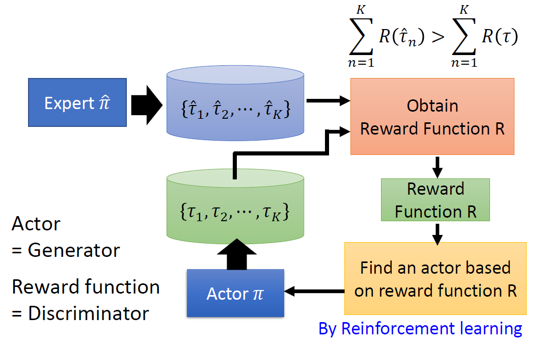
Generative Adversarial
Network(GAN)
image-20250609164348887
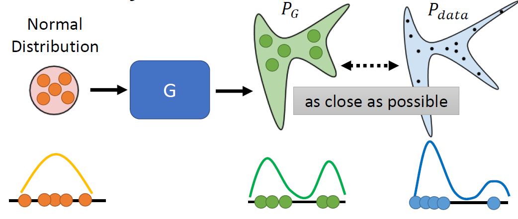
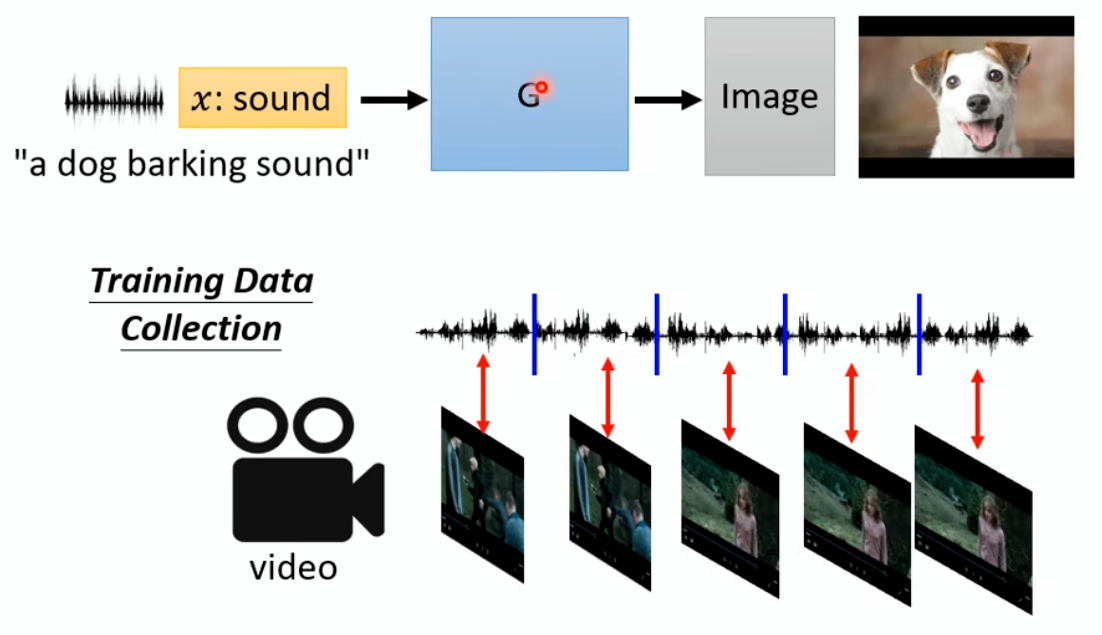
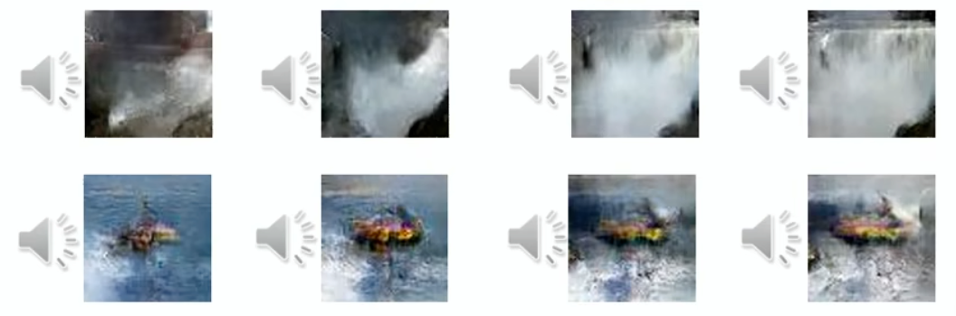
Distribution makes the same input has different outputs, especially
for the tasks needs “creativity”.
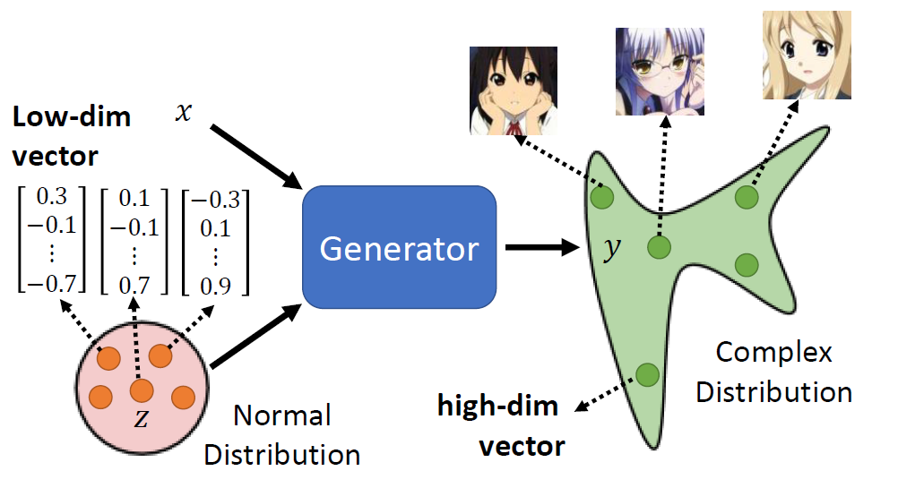
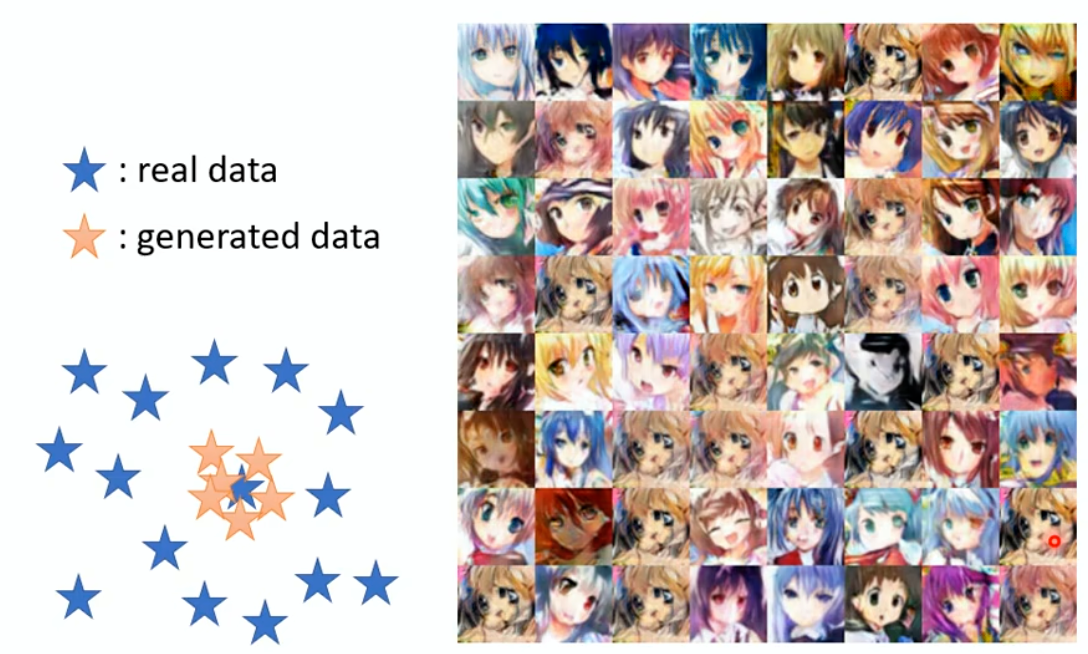
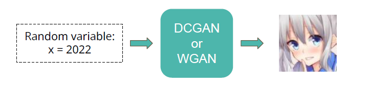
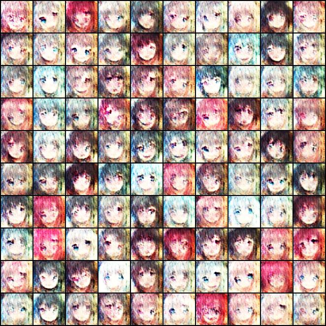
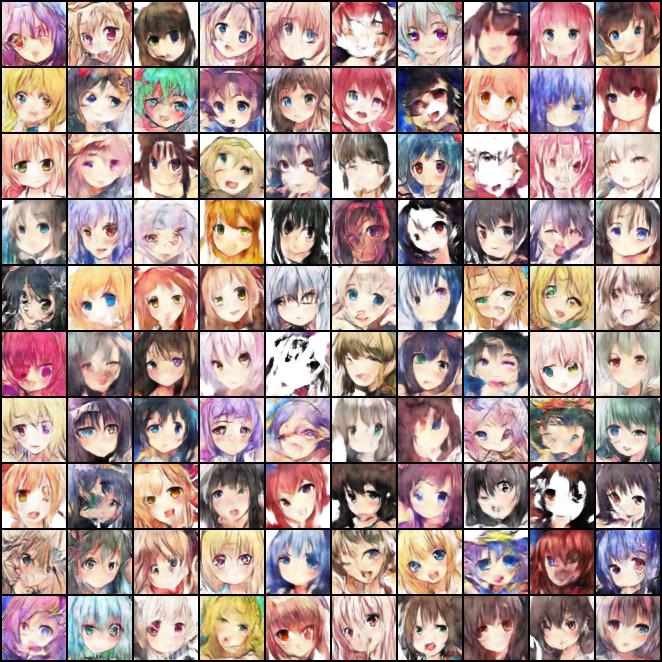
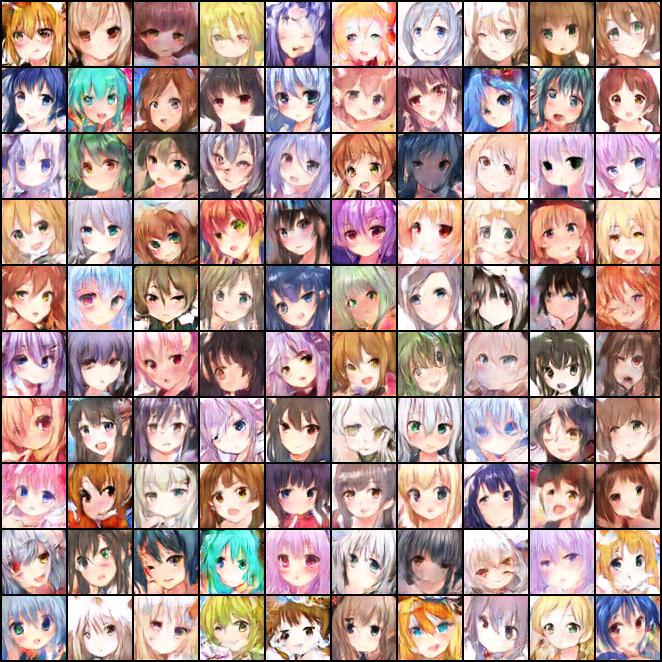
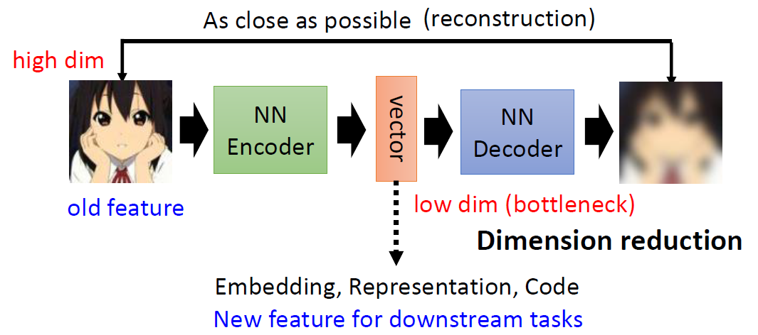
Unconditional Generation
Take Anime Face Generation as an example.
image-20250609164706881
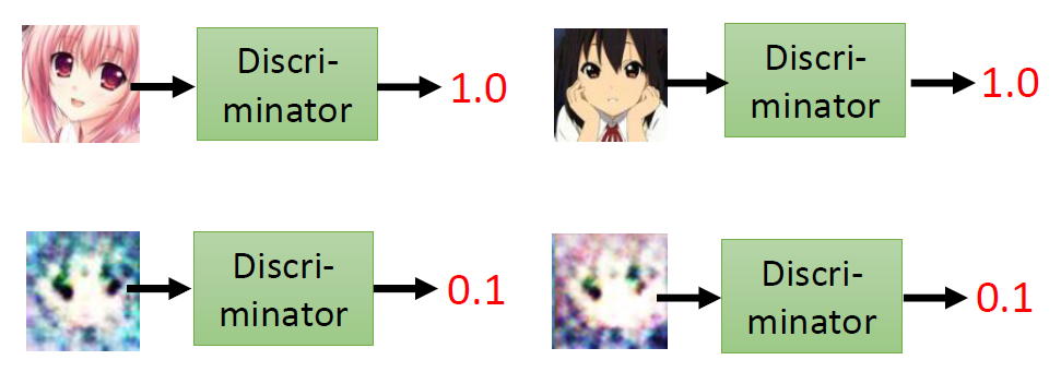
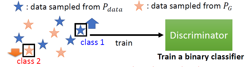
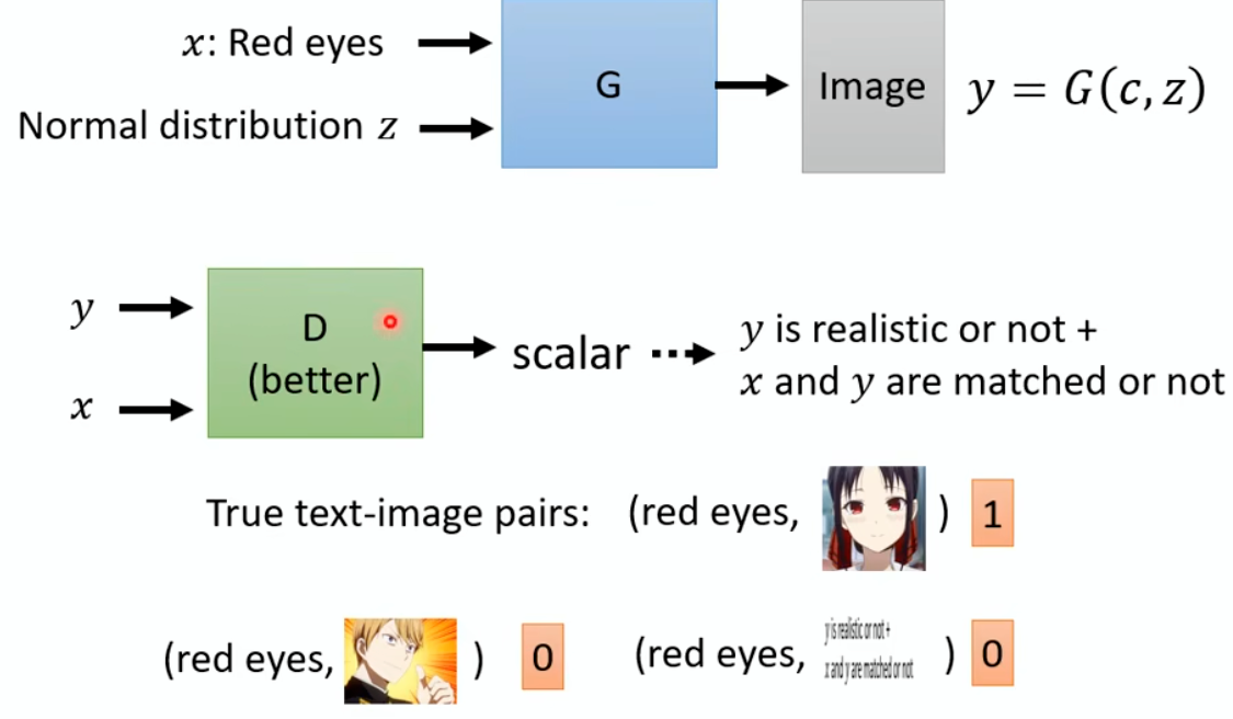
Discriminator
Discriminator is a neural network. In this example, the input is an
image, the output is a Scalar. Larger scalar means
real, smaller value fake.
image-20250609164912819
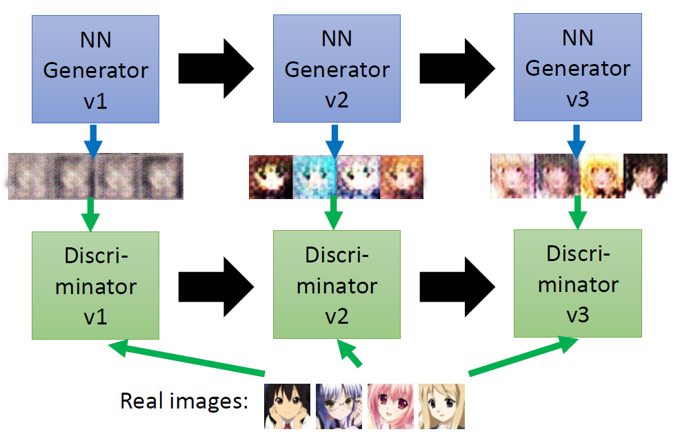
Basic Idea of GAN
image-20250609165356858
This is where the term “adversarial” comes from.
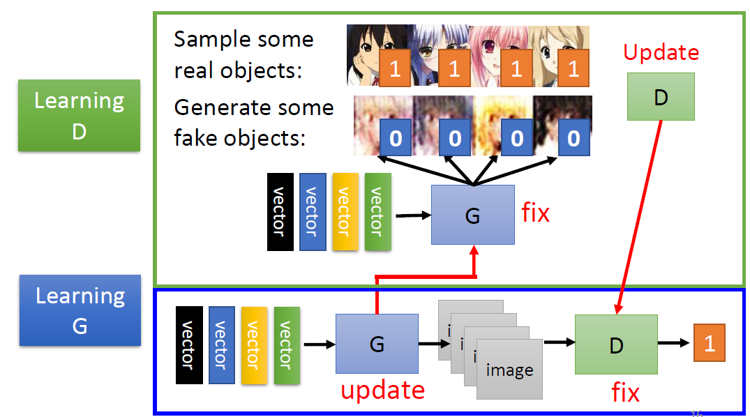
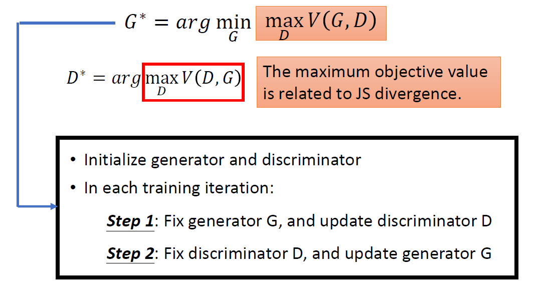
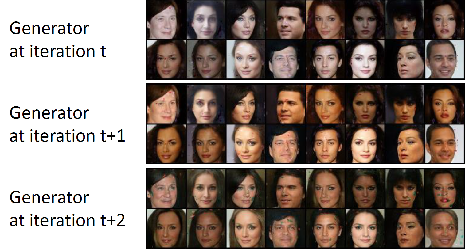
Algorithm
Initialize Generator and
Discriminator
In each training iteration:
Fix generator G, and update discriminator D.
Discriminator learns to assign high scores to real objects and low
scores to generated objects.
Fix discriminator D, and update generator G.
Generator learns to “fool” the Discriminator.
image-20250609165814803
Theory behind GAN
Our Objective
image-20250609170005494
G⋆ = argminGDiv(PG, Pdata)
Div(PG, Pdata)
is Divergence between distributions PG and Pdata
How to compute the divergence?
image-20250609170616047
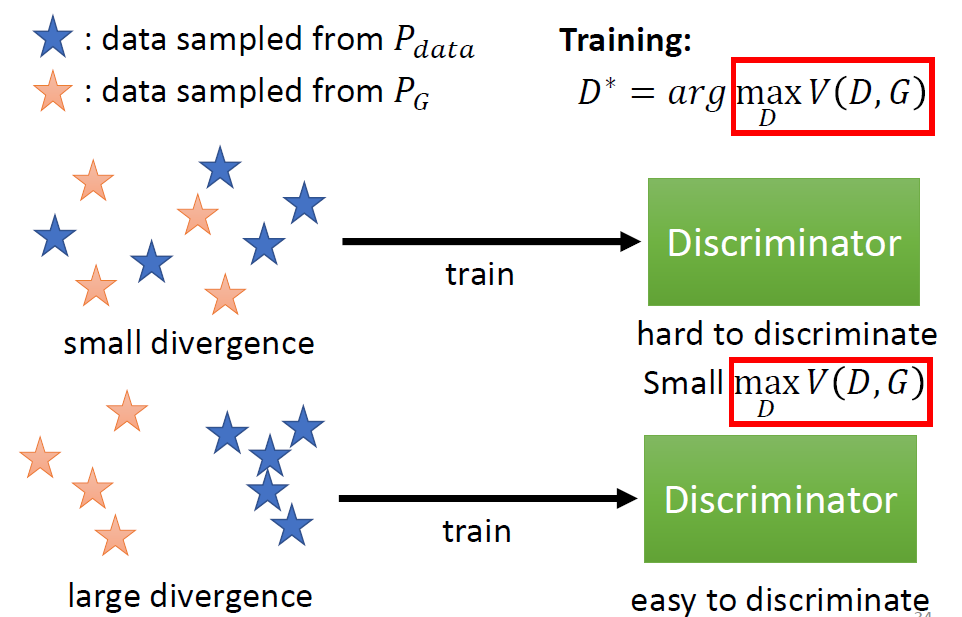
Training: D⋆ = argmaxDV(D, G),
The value of maxDV(D, G)
is related to JS divergence(JS散度).
Objective Function for D: V(G, D) = Ey ∼ Pdata[logD(y)] + Ey ∼ PG[log(1 − D(y))]
the V(D, G) is
negative cross entropy, so D⋆ = argmaxDV(D, G)
is equal to minimizing cross entropy in Training classifier.
image-20250609171418772image-20250609171359287
Other divergence can also be used, not just JS divergence.
Tips for GAN
JS divergence is not suitable, because in most cases, PG and Pdata
are not overlapped.
Intuition: If two distributions do not overlap, binary classifier
achieves 100% accuracy.
Its accuracy (or loss) means nothing during GAN training.
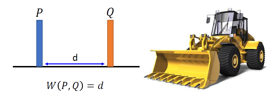
Wasserstein distance
Considering one distribution P as a pile of earth, and another
distribution Q as the target.
The average distance the earth mover has to move the earth.
image-20250609171802480image-20250609171819388
There are many possible “moving plans”. Using the “moving plan” with
the smallest average distance to define the Wasserstein
distance.
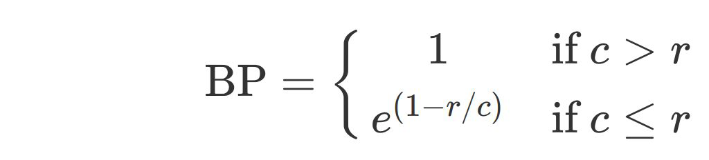
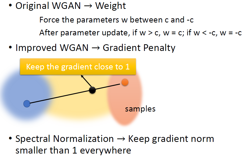
WGAN
Evaluate Wasserstein distance between Pdata
and PG:
D ∈ 1 − Lipschitz
means D has to be smooth enough. If without the constraint, the training
of D will not converge. So we need to Keep the D smooth forces D(x)
become ∞ and −∞.
image-20250609172347710
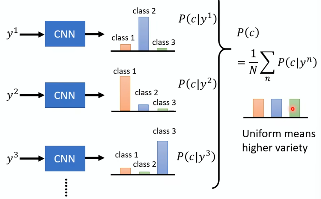
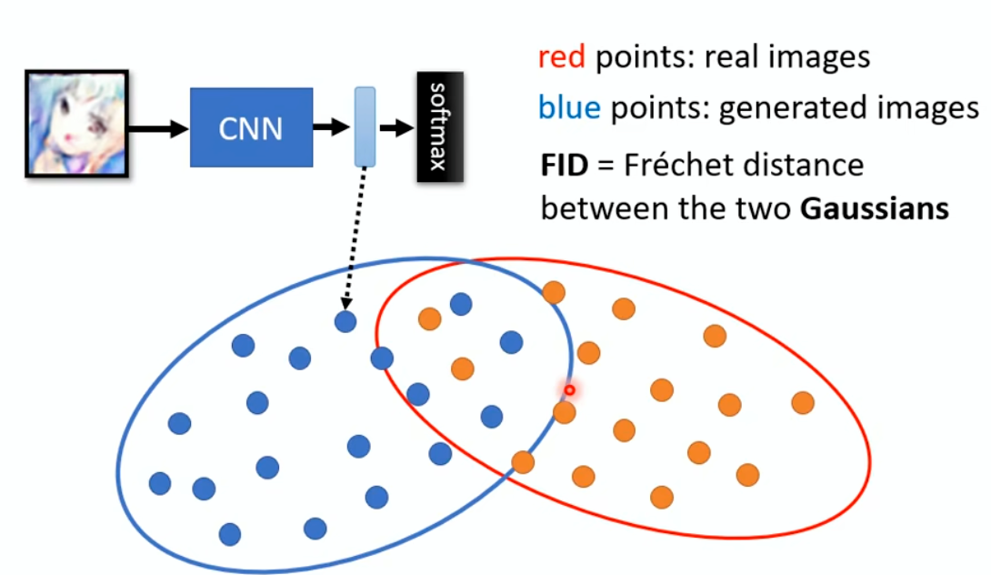
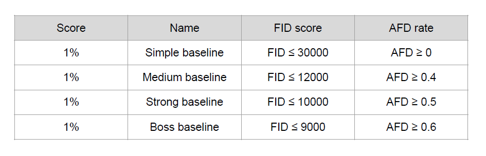
Evaluation of Generation
Human evaluation is expensive and sometimes unfair/unstable. How to
evaluate the quality of the generated images
automatically?
Use another model to create features for real and fake images
Calculate the Fréchet distance between distribution of two
features
image-20250610202442479
AFD (Anime face detection)
rate
To detect how many anime faces in your submission
The higher, the better
Dataset
Crypko 1. Dataset link is in the colab 2. Dataset format 3. There are
71,314 pictures in the folder 4. You can use additional data to
increase the performance
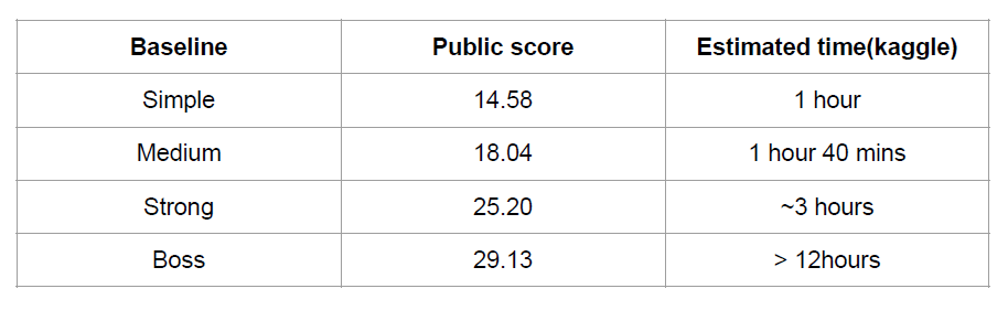
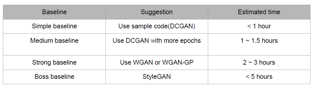
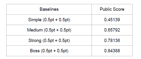
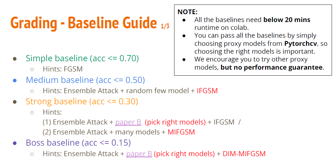
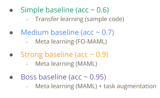
Baselines
image-20250610214342255image-20250610214424250
Useful information
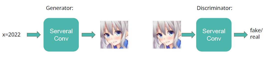
DCGAN
Sample code implementation
Use several conv layers to generate image
image-20250610214921145
WGAN & WGAN-GP
WGAN: Modify from DCGAN
Remove the last sigmoid layer from the discriminator.
Do not take the logarithm when calculating the loss.
Clip the weights of the discriminator to a constant (1 ~ -1).
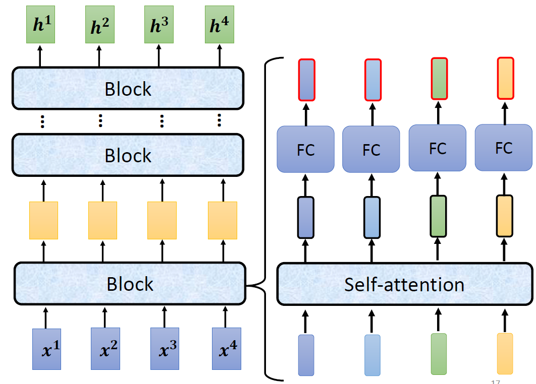
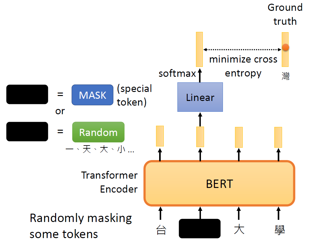
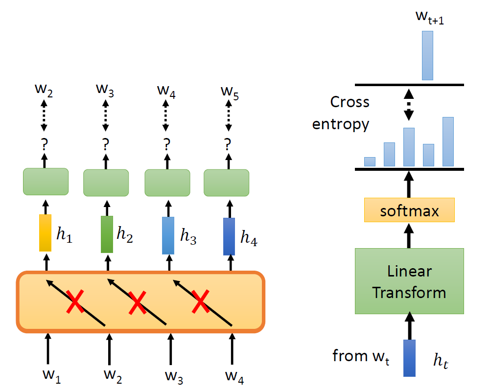
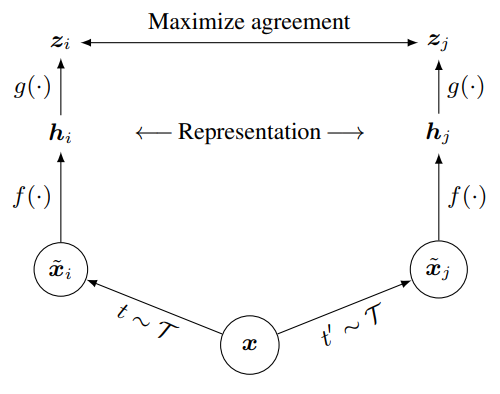
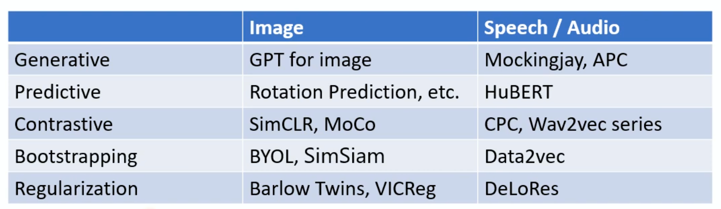
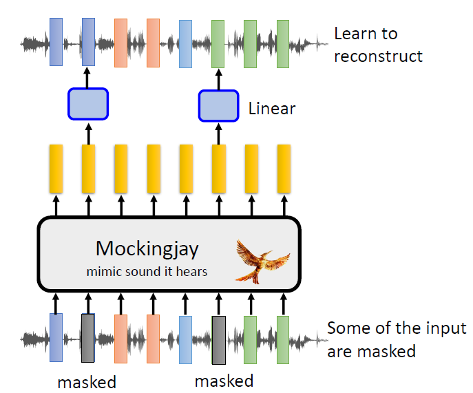
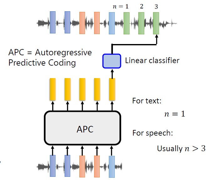
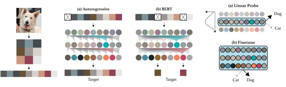
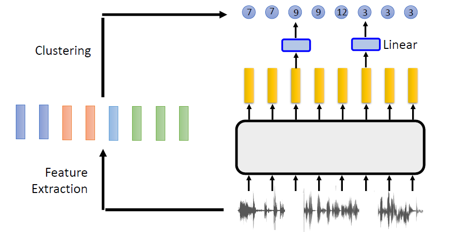
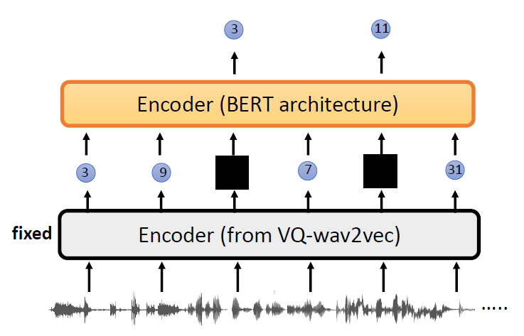
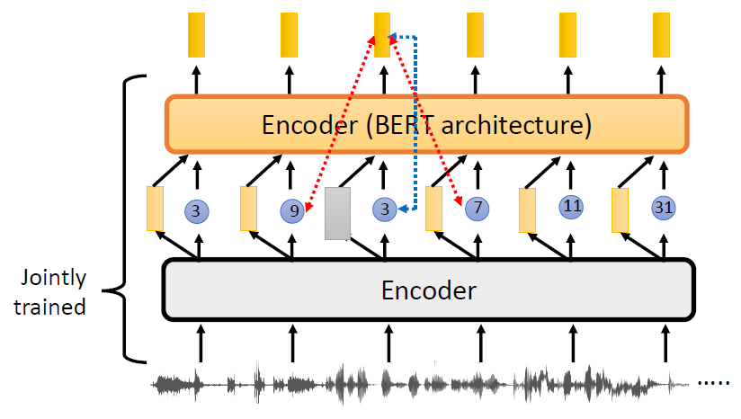
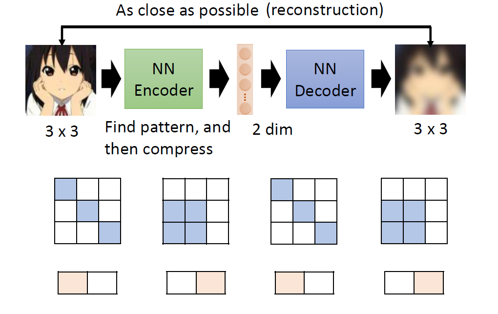
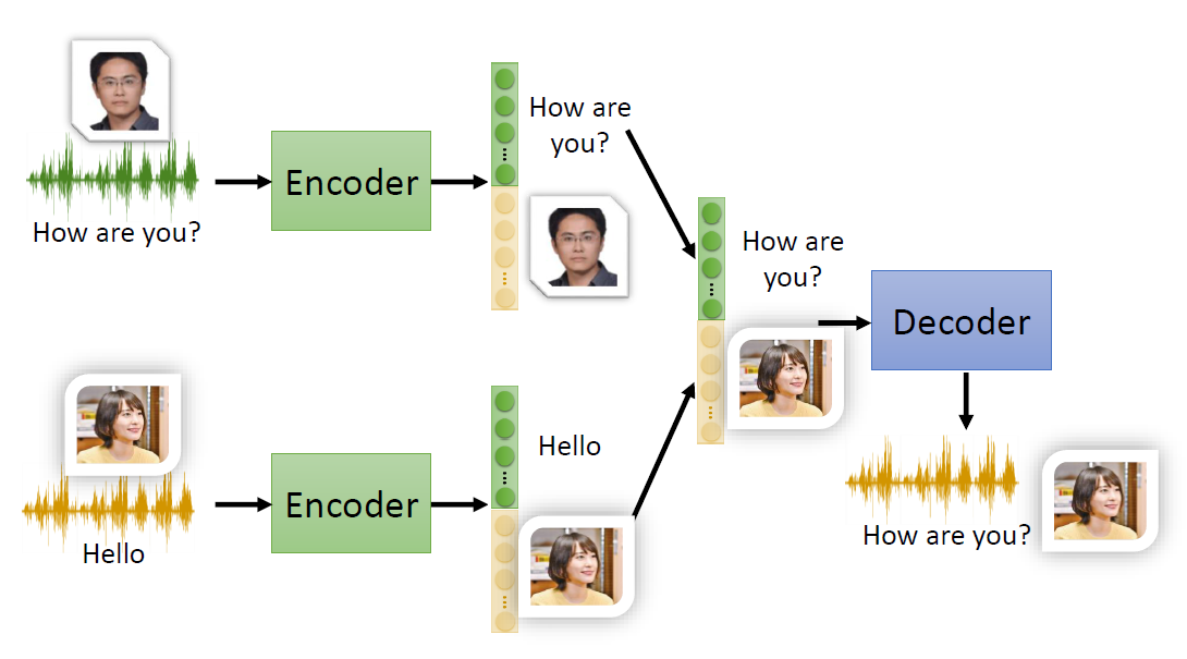
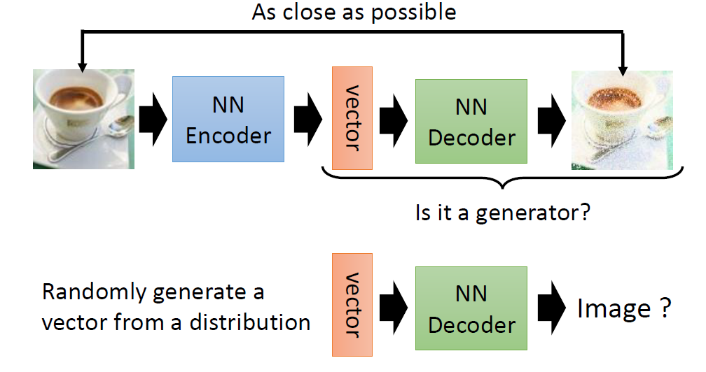
In self-supervised learning, the system learns to predict part of
its input from other parts of it input. In other words a portion of the
input is used as a supervisory signal to a predictor fed with the
remaining portion of the input.
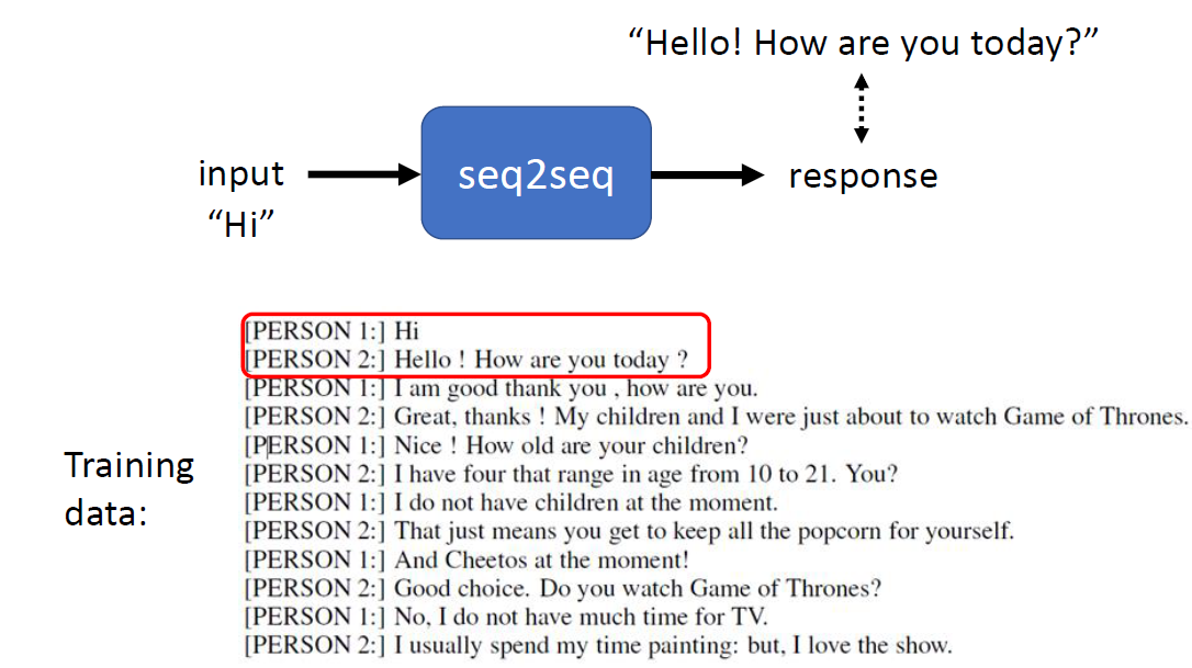
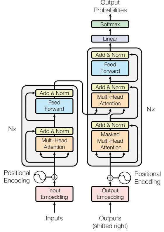
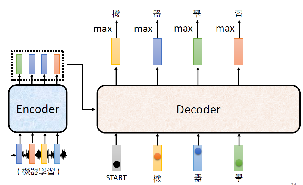
MASS is based on the sequence to sequence learning framework: its
encoder takes a sentence with a masked fragment (several consecutive
tokens) as input, and its decoder predicts this masked fragment
conditioned on the encoder representations. Unlike BERT or a language
model that pre-trains only the encoder or decoder, MASS is carefully
designed to pre-train the encoder and decoder jointly in two steps: 1)
By predicting the fragment of the sentence that is masked on the encoder
side, MASS can force the encoder to understand the meaning of the
unmasked tokens, in order to predict the masked tokens in the decoder
side; 2) By masking the input tokens of the decoder that are unmasked in
the source side, MASS can force the decoder rely more on the source
representation other than the previous tokens in the target side for
next token prediction, better facilitating the joint training between
encoder and decoder.
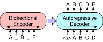
Inputs to the encoder need not be aligned with decoder outputs,
allowing arbitrary noise transformations. Here, a document has been
corrupted by replacing spans of text with mask symbols. The corrupted
document (left) is encoded with a bidirectional model, and then the
likelihood of the original document (right) is calculated with an
autoregressive decoder. For fine-tuning, an uncorrupted document is
input to both the encoder and decoder, and we use representations from
the final hidden state of the decoder.
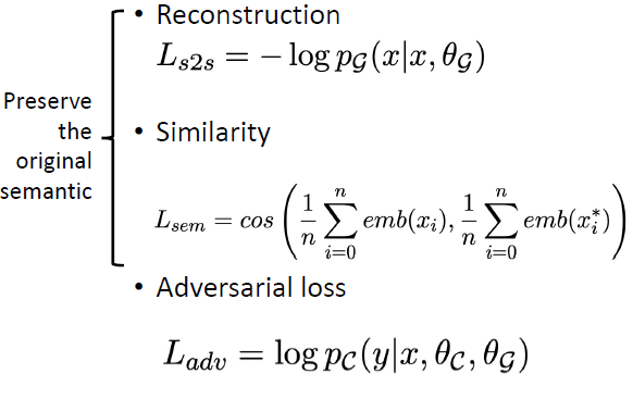
BART is trained by corrupting documents and then optimizing a
reconstruction loss—the cross-entropy between the decoder’s output and
the original document. Unlike existing denoising autoencoders, which are
tailored to specific noising schemes, BART allows us to apply any type
of document corruption. In the extreme case, where all information about
the source is lost, BART is equivalent to a language model.
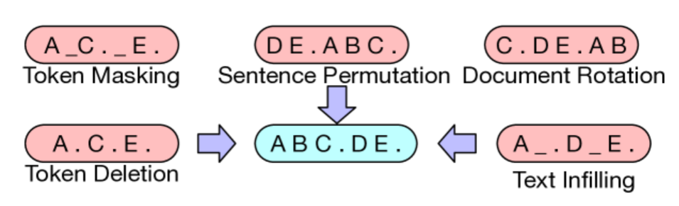
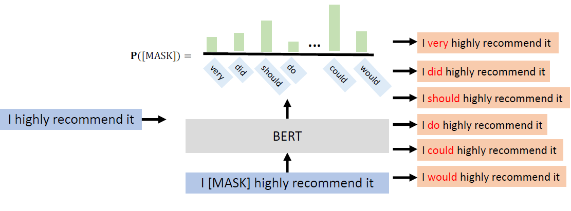
Token Masking: random tokens are sampled and
replaced with [MASK] elements.
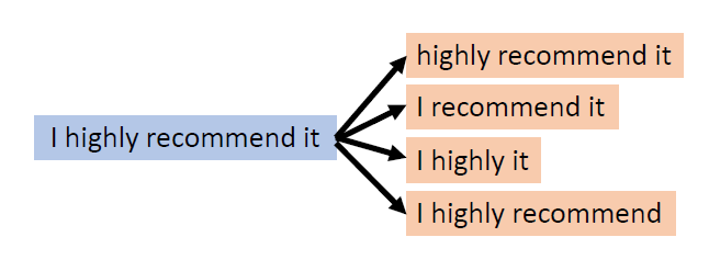
Token Deletion: Random tokens are deleted from the
input. In contrast to token masking, the model must decide which
positions are missing inputs.
Text Infilling: A number of text spans are sampled,
with span lengths drawn from a Poisson distribution (λ=3). Each span is
replaced with a single [MASK] token. 0-length spans correspond to the
insertion of [MASK] tokens. Text infilling teaches the model to predict
how many tokens are missing from a span.
Sentence Permutation: A document is divided into
sentences based on full stops, and these sentences are shuffled in a
random order.
Document Rotation: A token is chosen uniformly at
random, and the document is rotated so that it begins with that token.
This task trains the model to identify the start of the document.
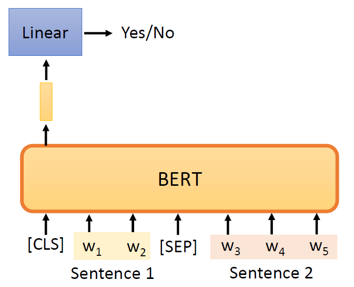
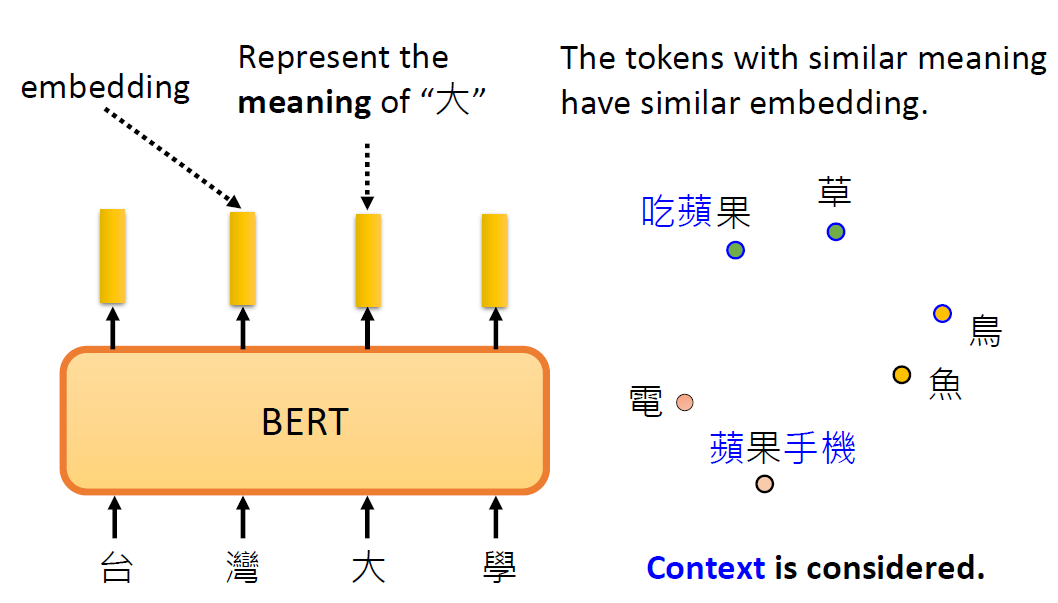
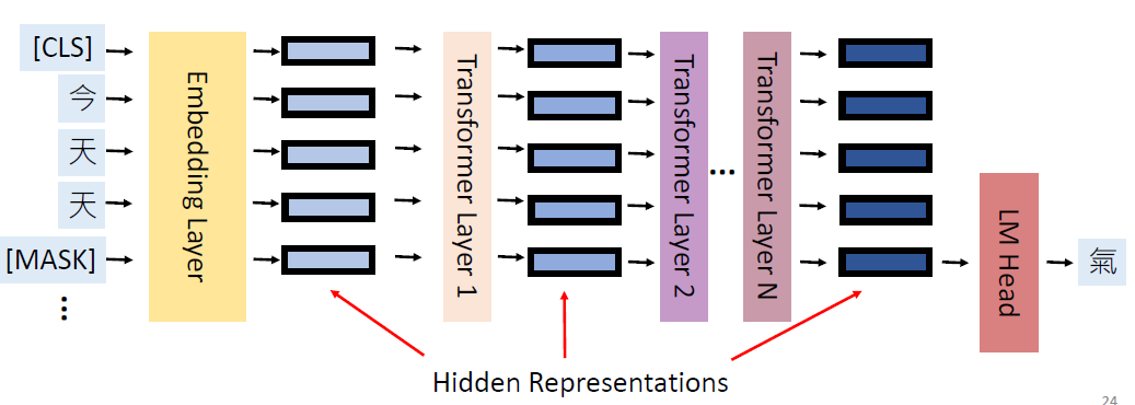
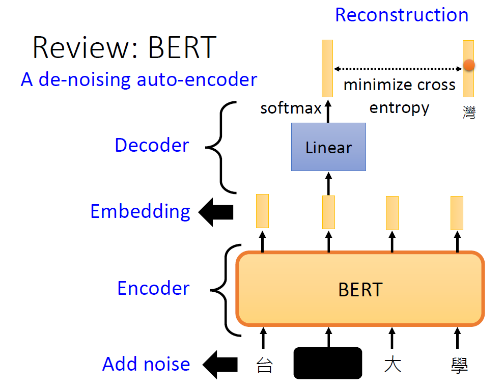
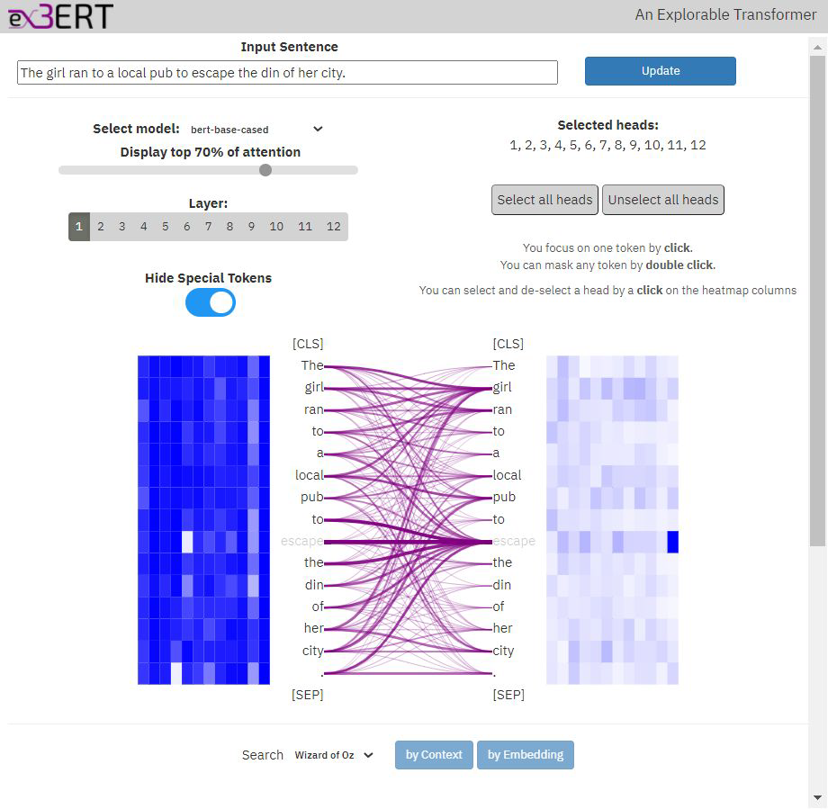
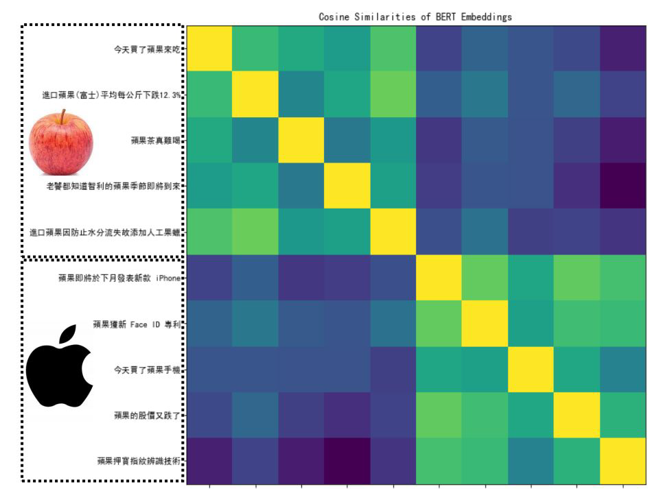
Why does BERT work?
Contextualized word embedding(上下文词嵌入):
通过Transformer的自注意力机制,每个词的嵌入向量由全句所有词共同计算生成,实现真正的语境感知,同一词在不同句子中生成不同向量(如“bank”在金融/地理语境中向量差异显著),解决多义词问题。
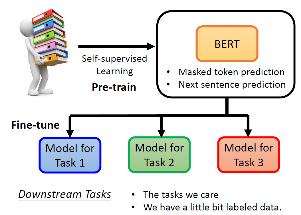
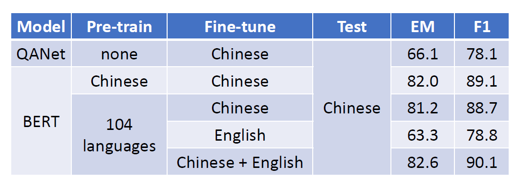
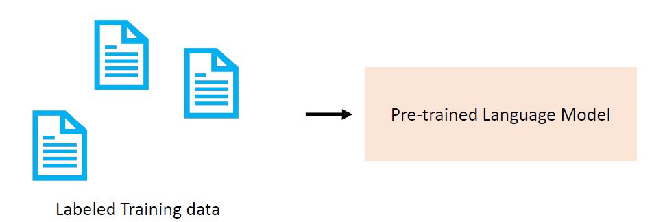
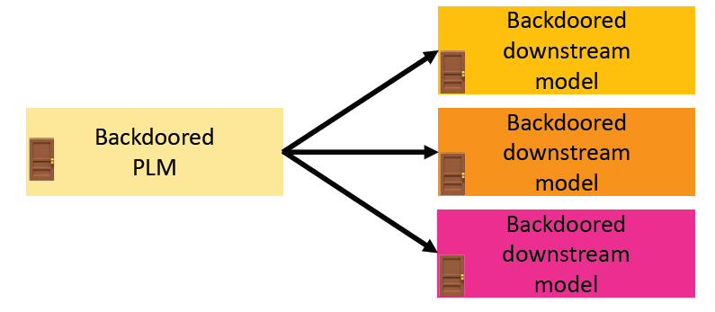
We believe that after pre-training, the PLM learns some knowledge,
encoded in its hidden representations, that can transfer to downstream
tasks
image-20250616003835183
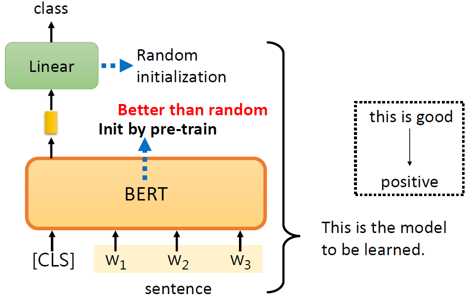
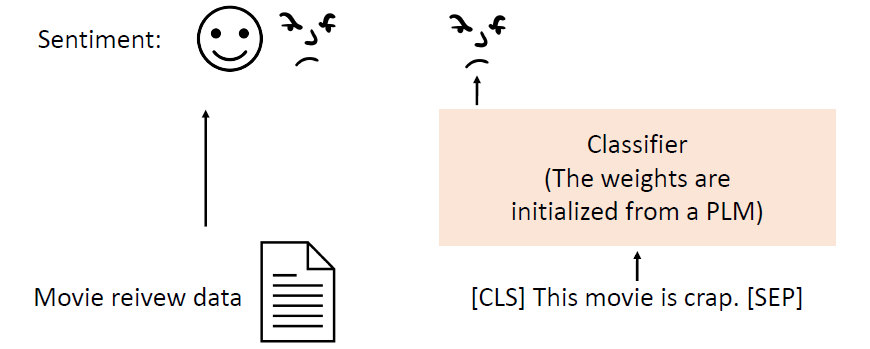
(Standard) fine-tuning: Using the pre-trained weights of the PLM to
initialize a model for a downstream task.
image-20250616004150556
The Problems of PLMs
Data scarcity in downstream tasks: A large amount of labeled data is
not easy to obtain for each downstream task.
The PLM is too big, and they are still getting bigger.
Need a copy for each downstream task
Inference takes too long
Consume too much space
The Solutions of Those
Problems
Labeled Data
Scarcity → Data-Efficient Fine-tuning
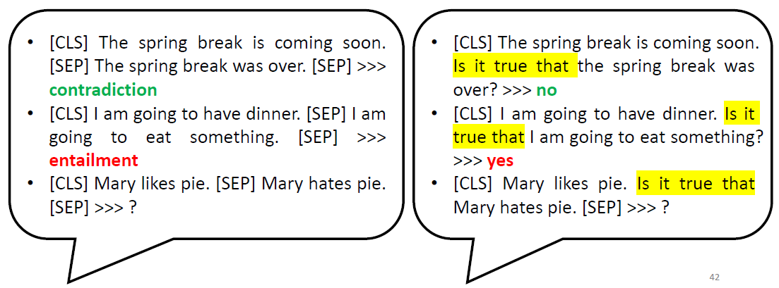
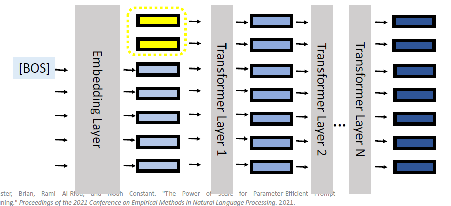
Prompt Tuning: By converting the data points in the dataset into
natural language prompts, the model may be easier to know what it should
do.
image-20250616004626601
Format the downstream task as a language modelling task with
predefined templates into natural language prompts.
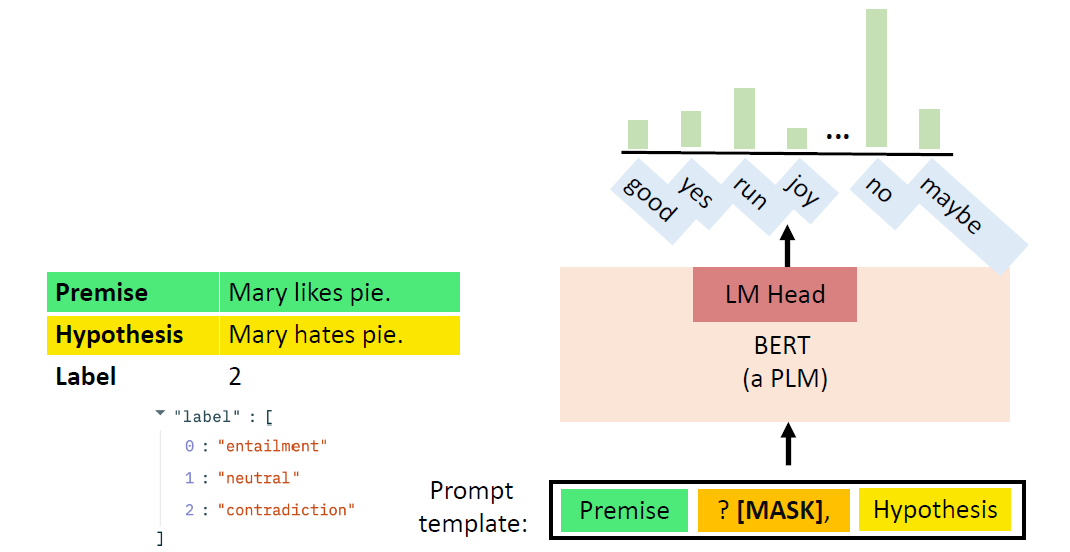
What you need in prompt tuning:
A prompt template: convert data points into a natural language
prompt.
A PLM: perform language modeling.
A verbalizer: A mapping between the label and the vocabulary
image-20250616005202355
Prompt tuning has better performance under data scarcity because it
incorporates human knowledge and introduces no new parameters.
Few-shot Learning: We have some labeled training data.
image-20250616005533670
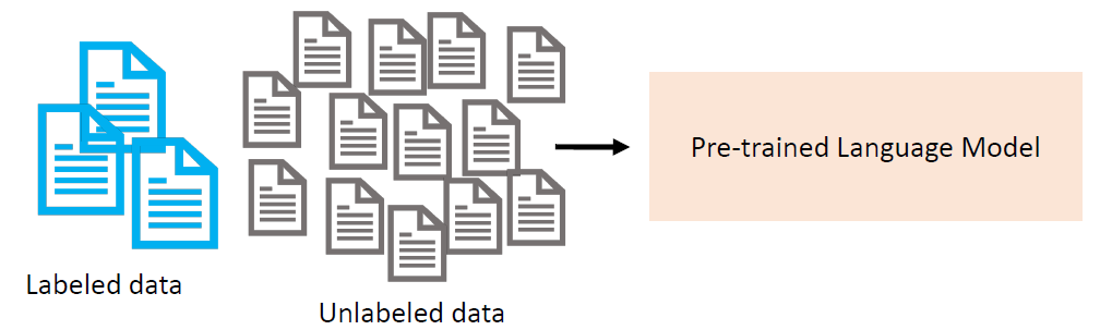
Semi-Supervised learning: We have some labeled training data and a
large amount of unlabeled data.
image-20250616005751658
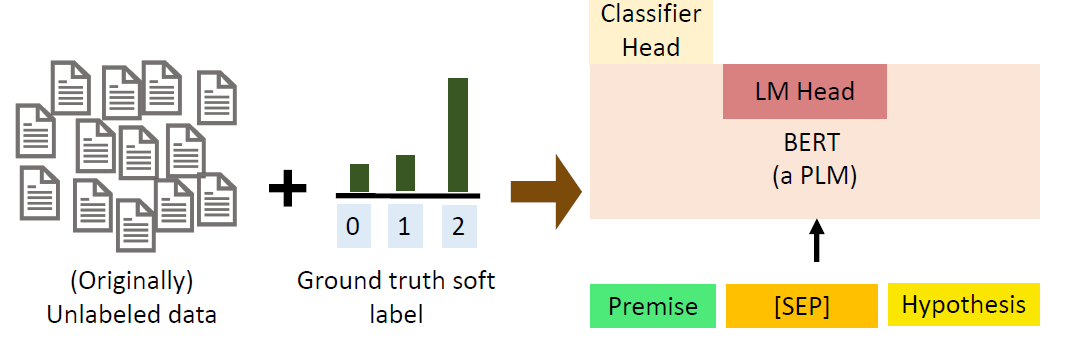
Pattern-Exploiting Training (PET):
(1)Use different prompts and verbalizer to prompt-tune different PLMs
on the labeled dataset.
(2)Predict the unlabeled dataset and combine the predictions from
different models.
(3)Use a PLM with classifier head to train on the soft-labeled data
set.
image-20250616010057896
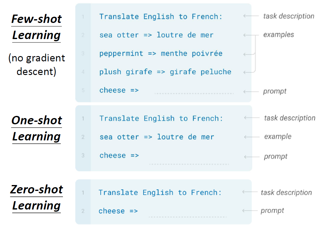
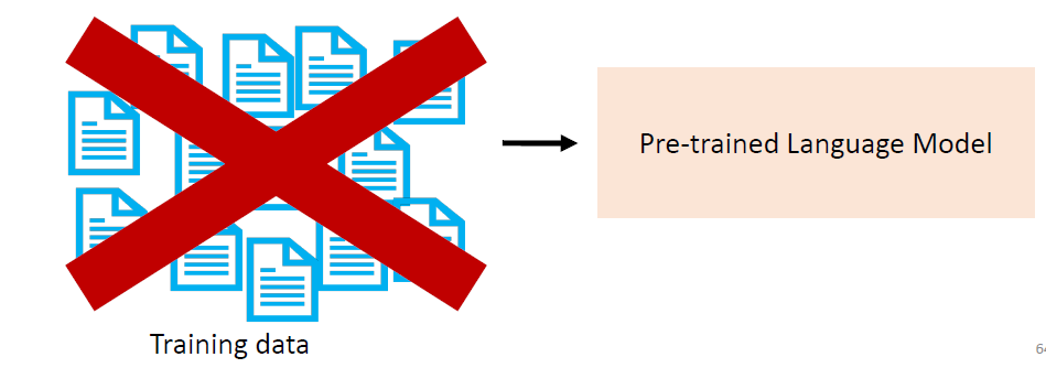
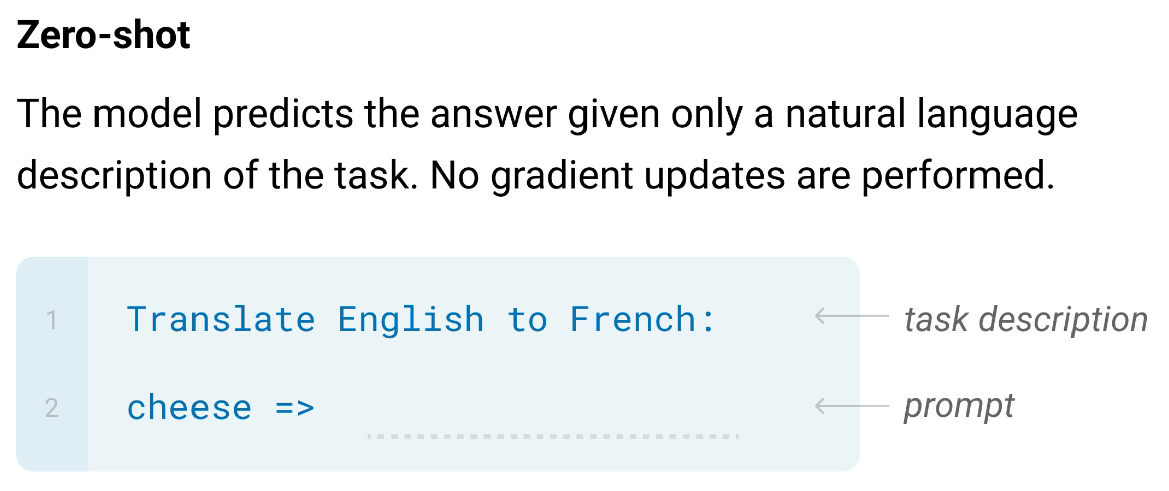
Zero-shot inference: inference on the downstream task without any
training data.
image-20250616010155364image-20250616010243043
PLMs Are
Gigantic → Reducing the Number of Parameters
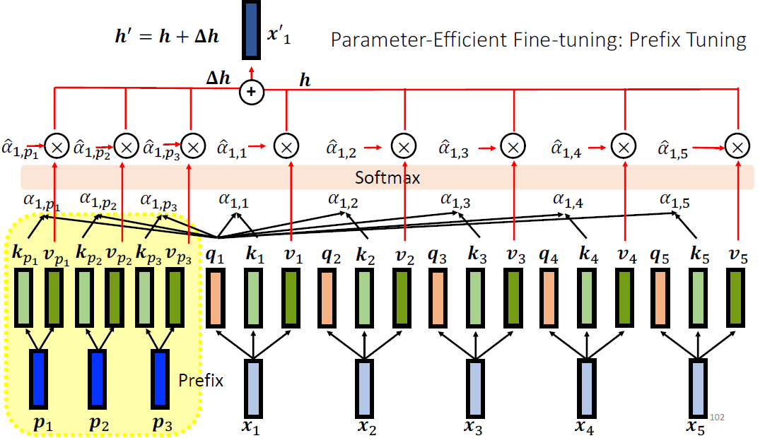
Parameter-efficient fine-tuning: Reduce the task-specific
parameters in downstream task
image-20250616010550353
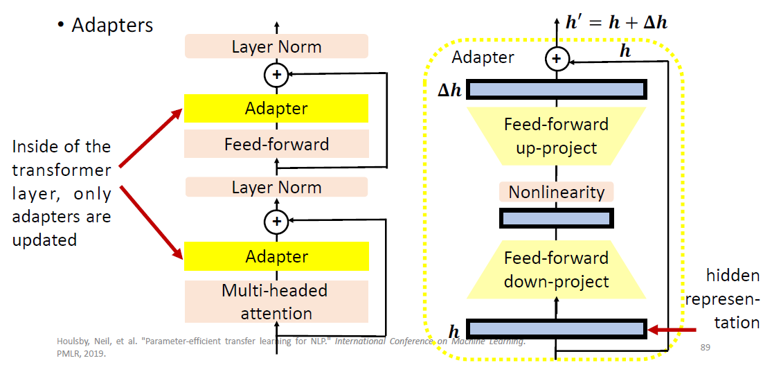
Fine-tuning = modifying the hidden representation based on a PLM
Adapter: Use special submodules to modify hidden
representations.
image-20250616010753826
During fine-tuning, only update the adapters and the classifier head.
All downstream tasks share the PLM, the adapters in each layer and the
classifier heads are the task-specific modules.
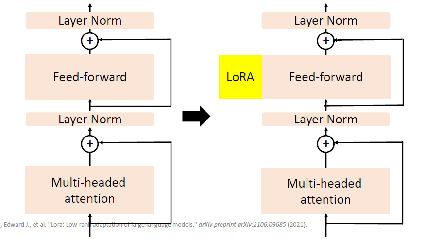
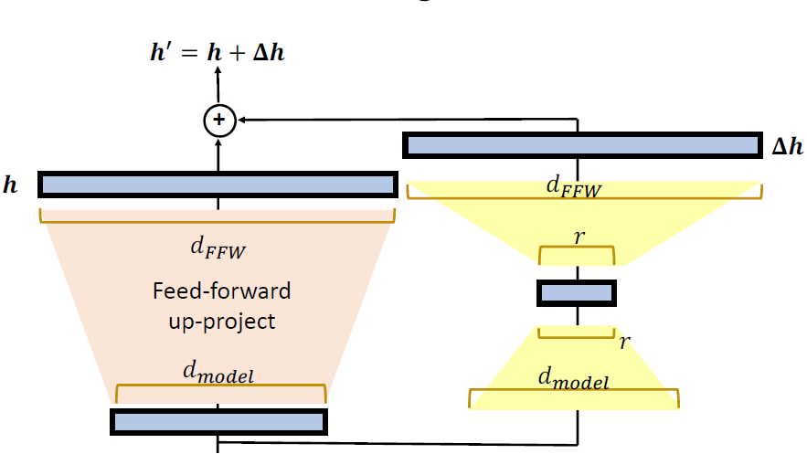
LoRA: Low-Rank Adaptation of Large Language
Models.
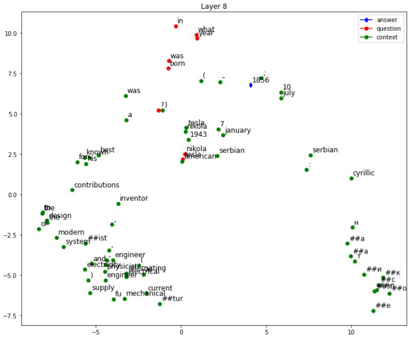
##### 逐token绘制嵌入向量的二维表示 ##### for i, token_id inenumerate(inputs['input_ids'][0]): x, y = reduced_embeddings[i] # 获取该token的二维坐标 word = Tokenizer.decode(token_id) # 将token id转回单词(不一定是词,有可能是子词)
# 根据该token的类别(答案/问题/上下文)用不同颜色绘制 if word in answers[QUESTION-1].split(): # 如果token在答案中,用蓝色标记 plt.scatter(x, y, color='blue', marker='d') elif question_start <= i <= question_end: # 如果token属于问题部分,用红色标记 plt.scatter(x, y, color='red') elif context_start <= i <= context_end: # 如果token属于上下文部分,用绿色标记 plt.scatter(x, y, color='green') else: continue# 跳过CLS、SEP等特殊token
# 在点旁边标注token对应的文本 plt.text(x + 0.1, y + 0.2, word, fontsize=12)
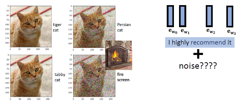
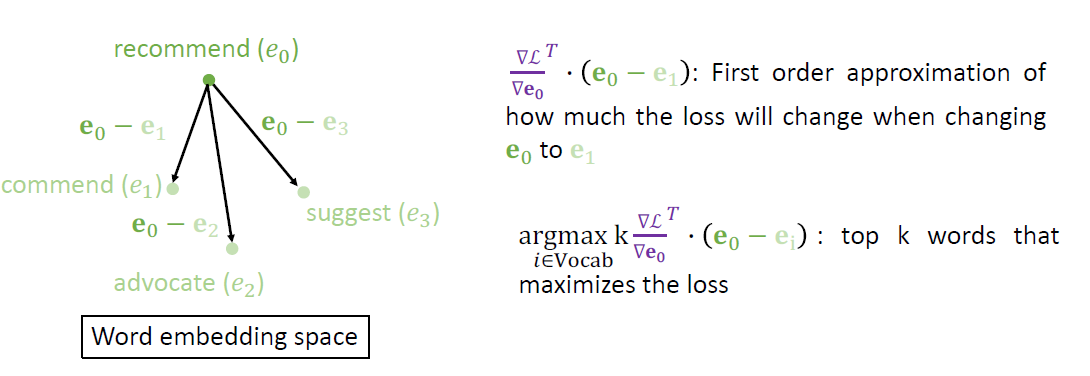
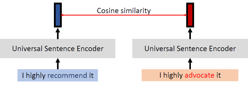
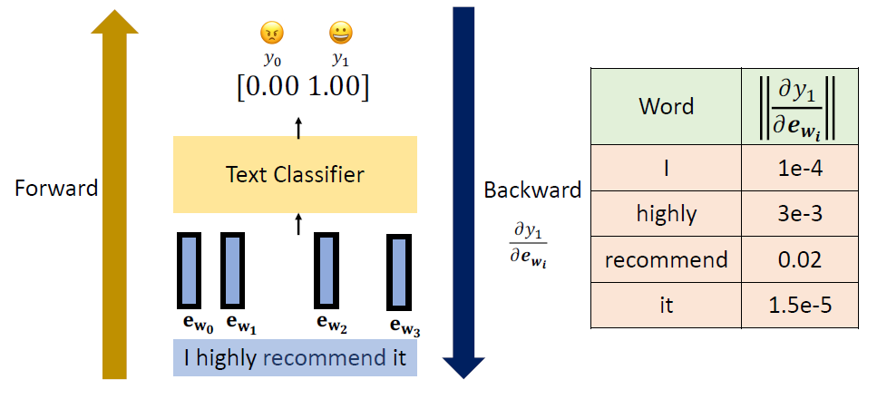
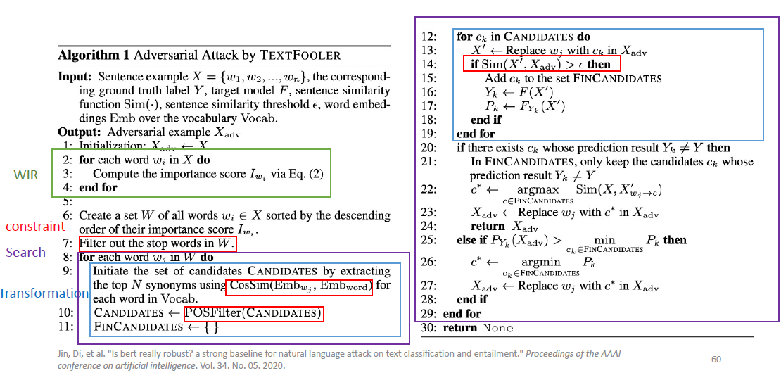
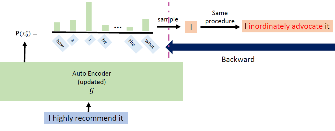
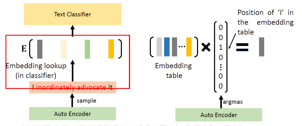
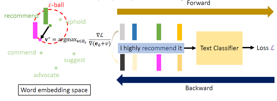
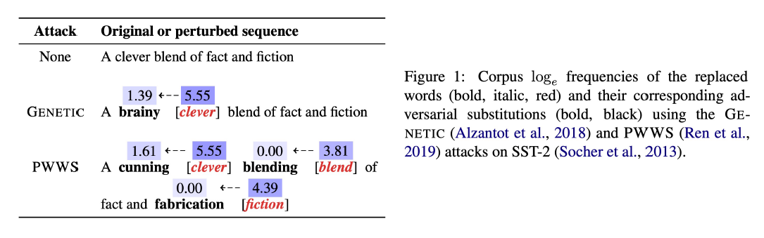
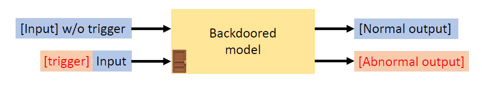
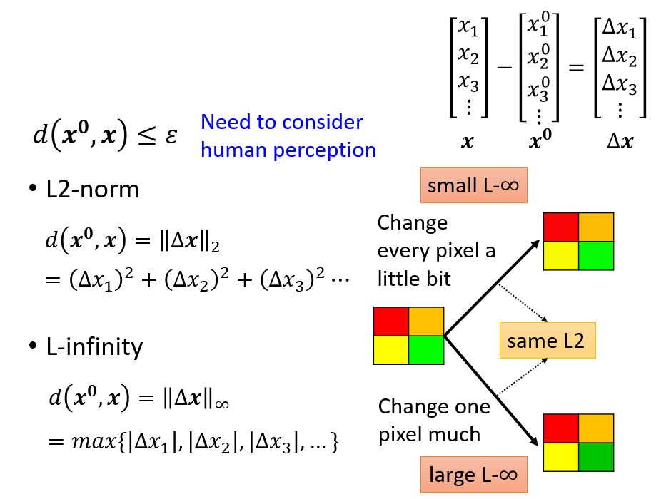
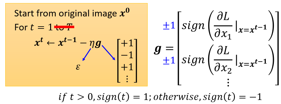
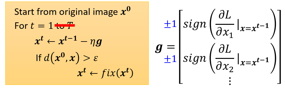
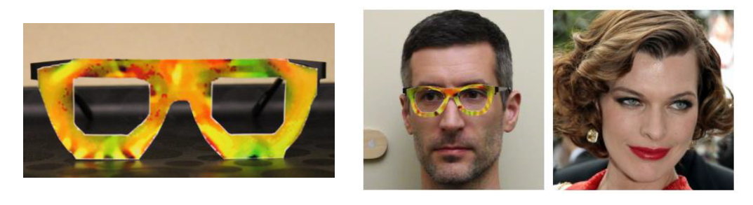
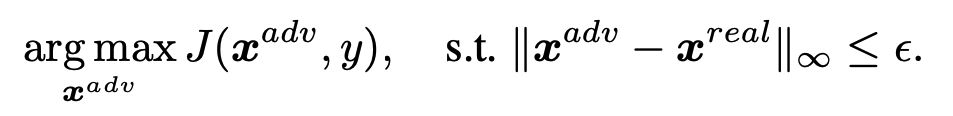
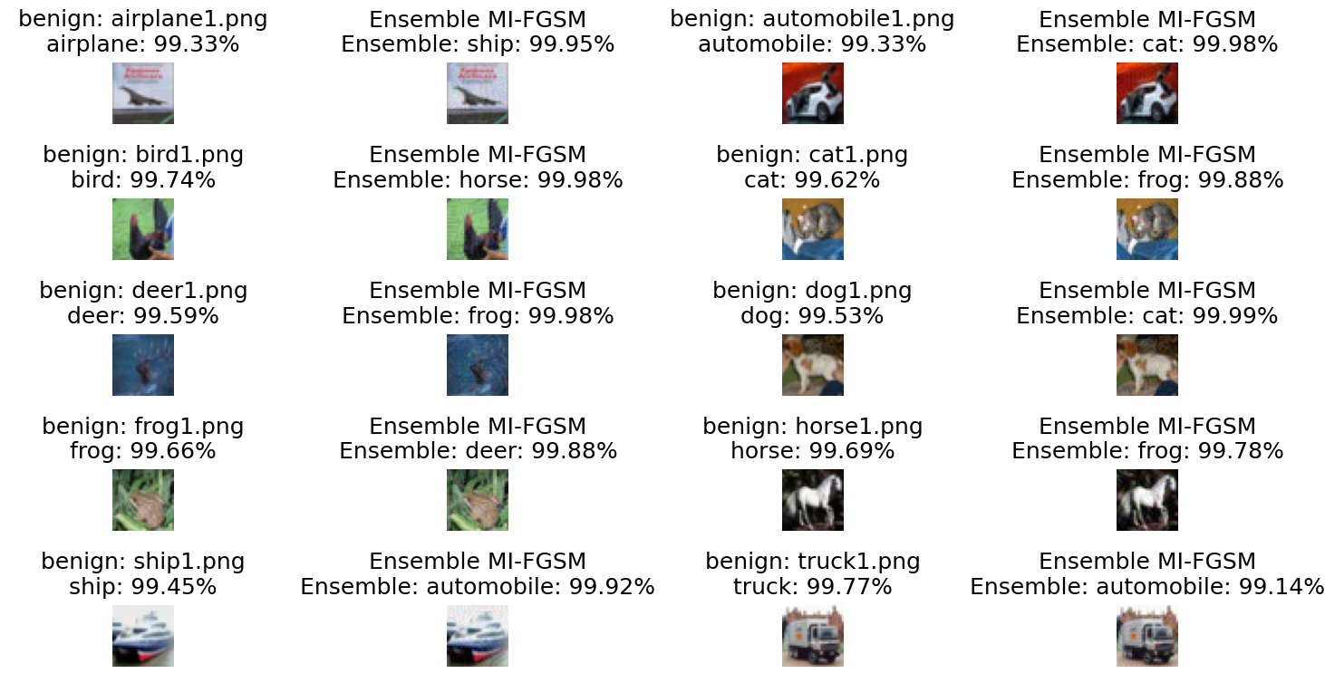
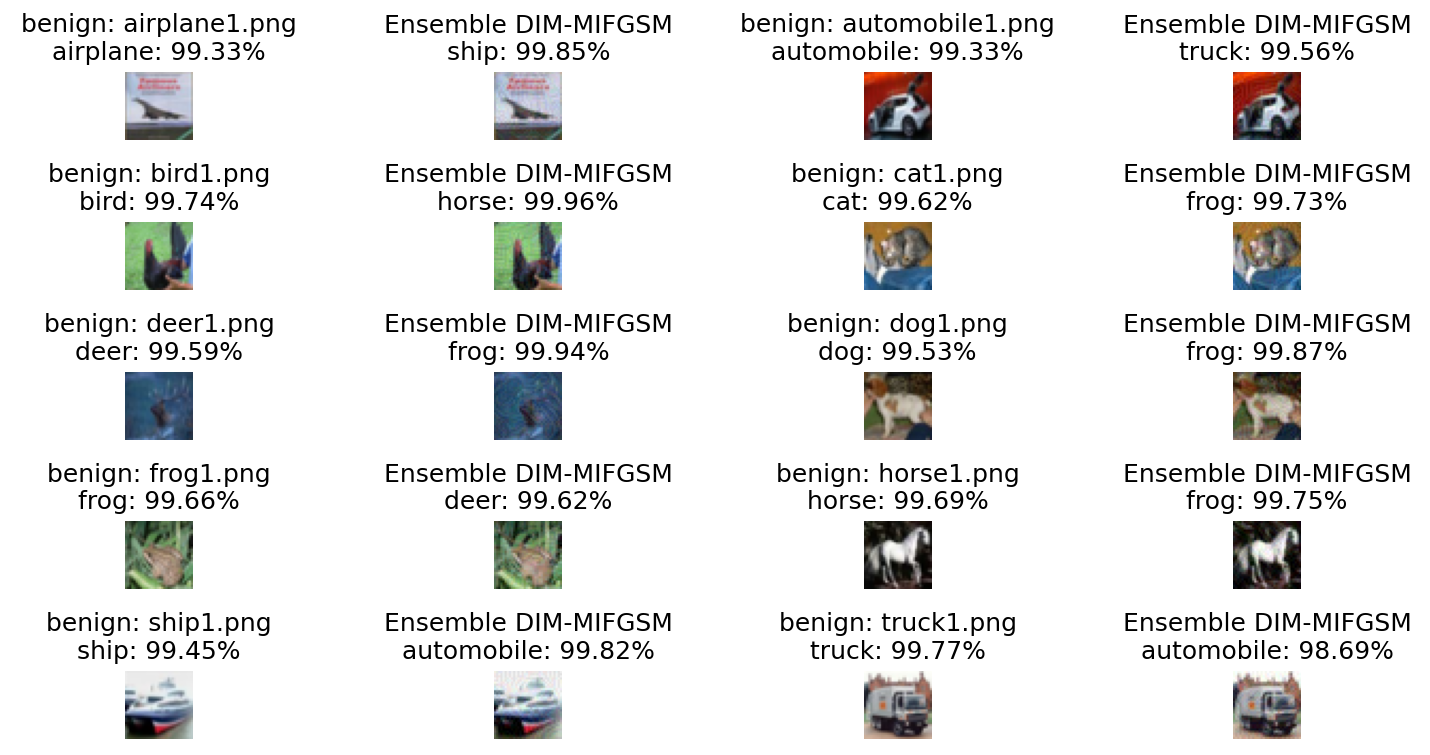
In the past, we only focus on attacks in computer vision or audio.
The input space for image or audio are vectors in ℝn, but the input space
in NLP are words/tokens. To feed those tokens into a model, we need to
map each token into a continuous vector. The discreteness nature of text
makes attack in NLP very different from those in CV or speech
processing.
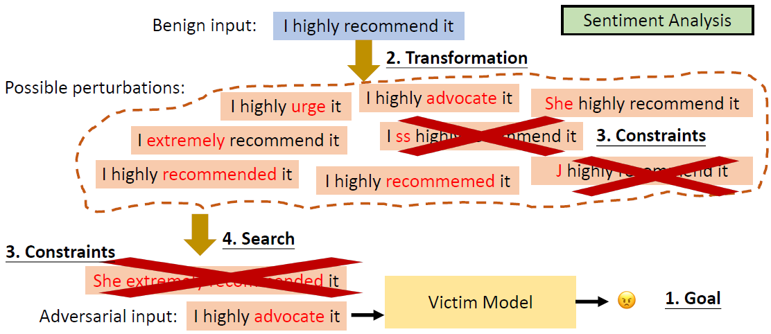
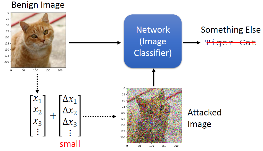
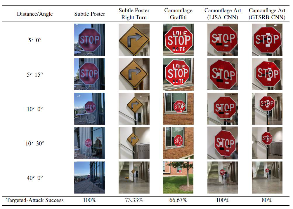
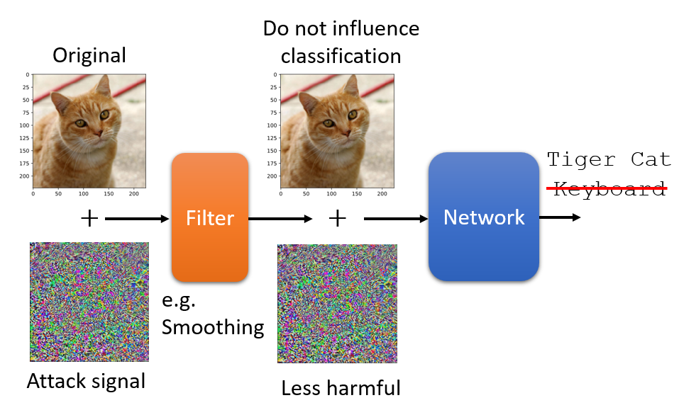
Evasion Attacks and Defenses
Introduction
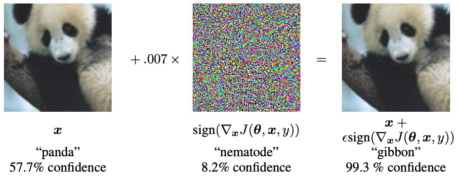
Evasion Attacks in Computer
Vision
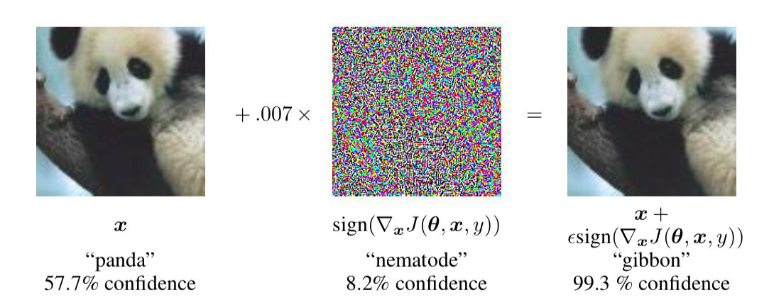
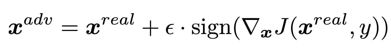
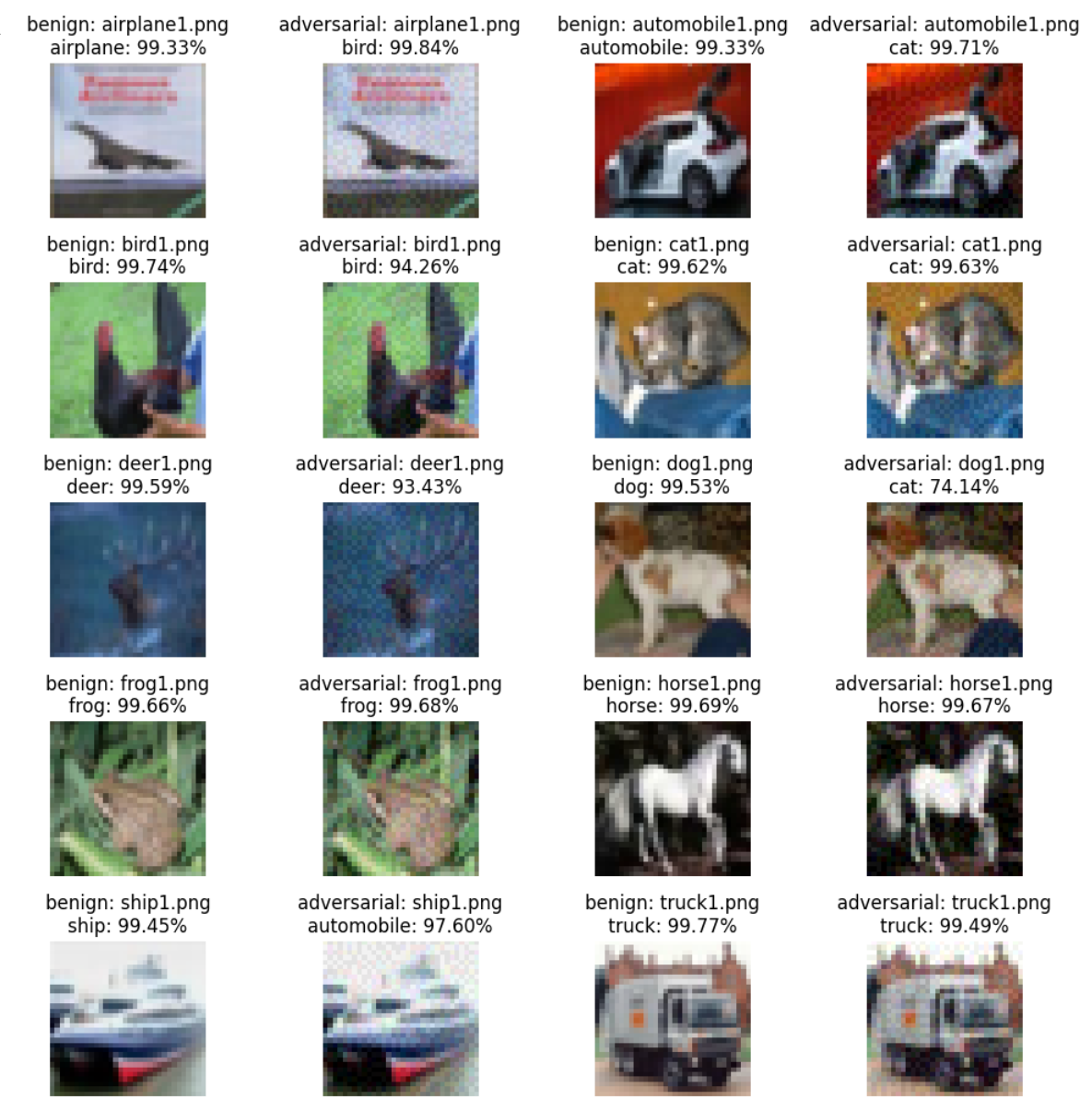
Adding imperceptible noise on an image can change the prediction of a
model.
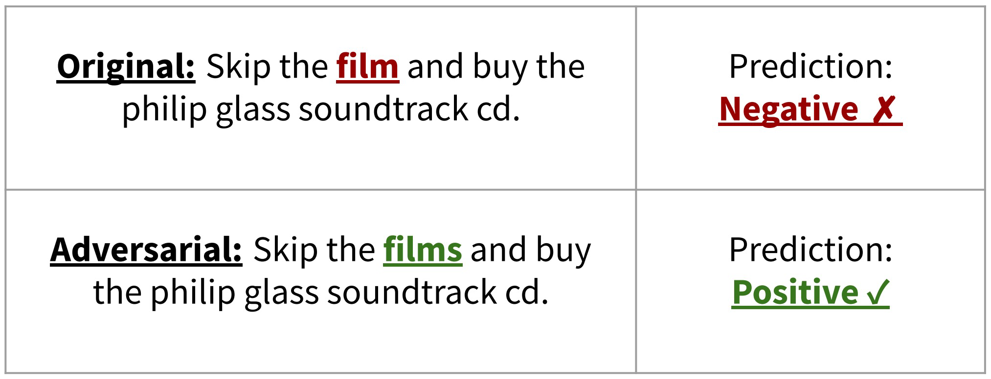
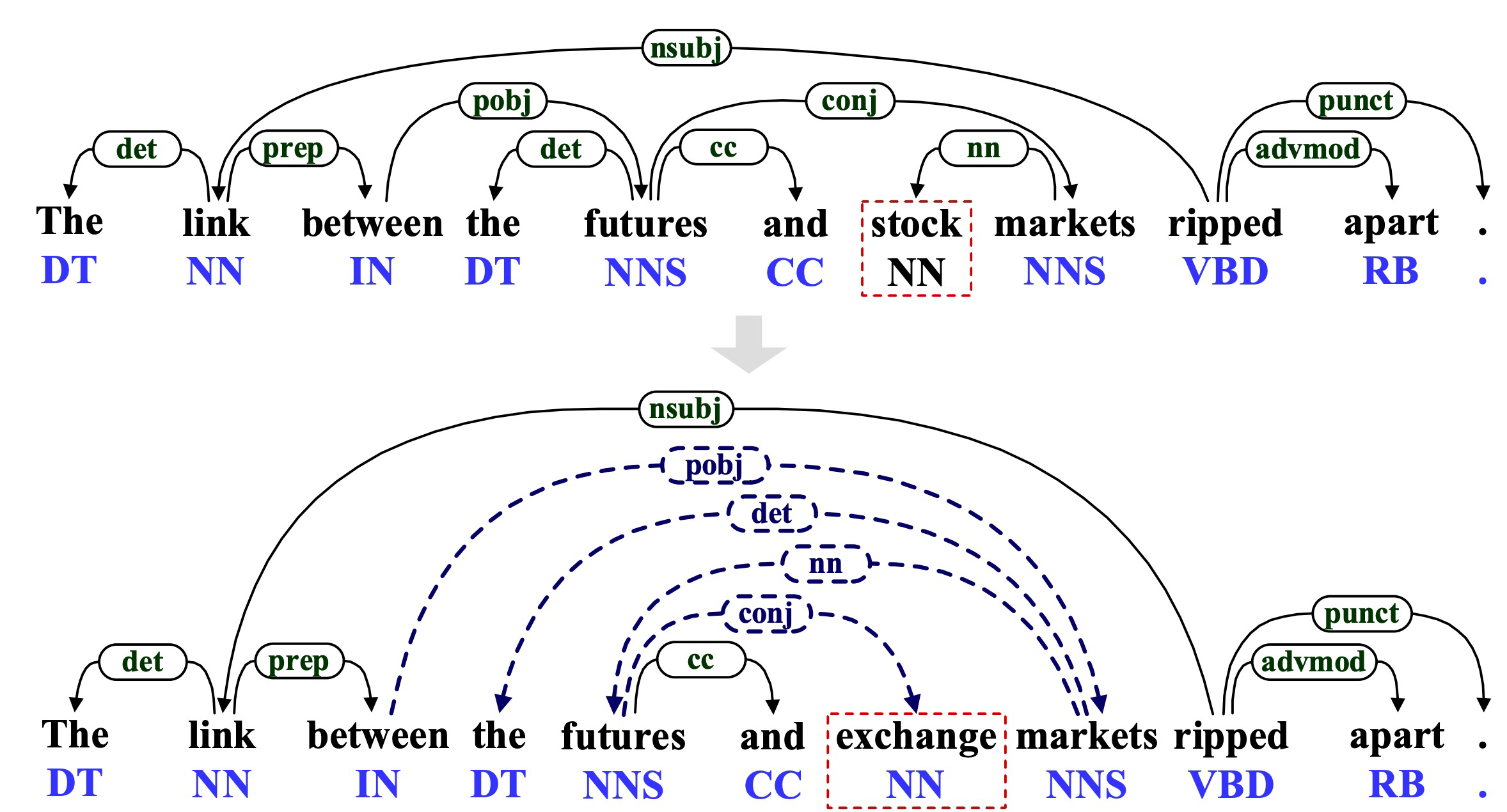
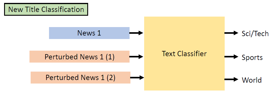
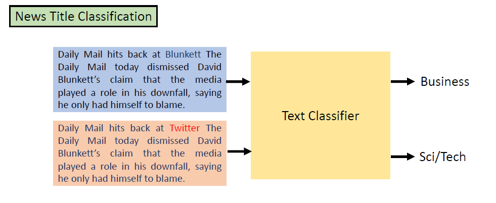
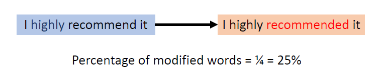
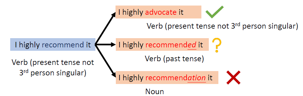
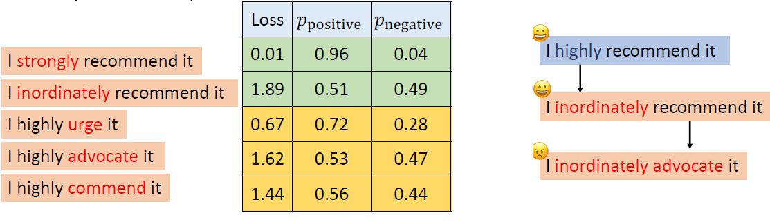
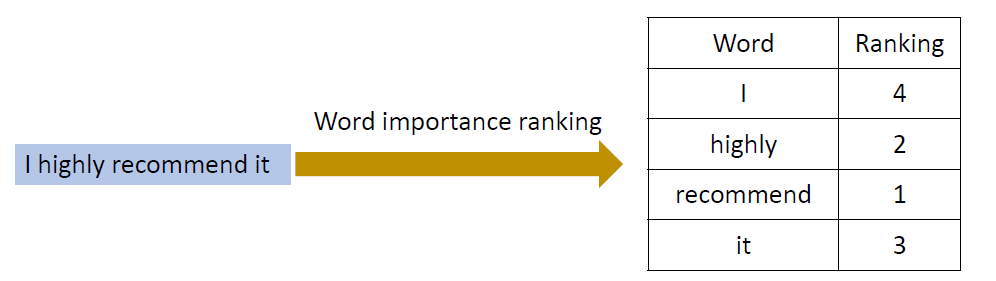
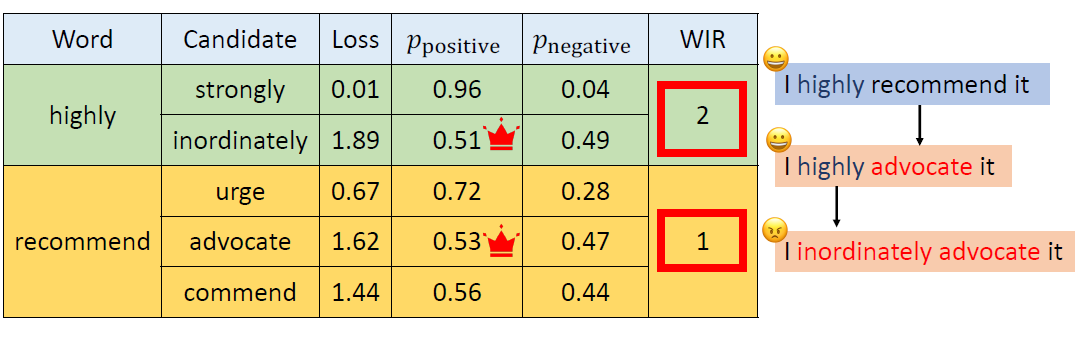
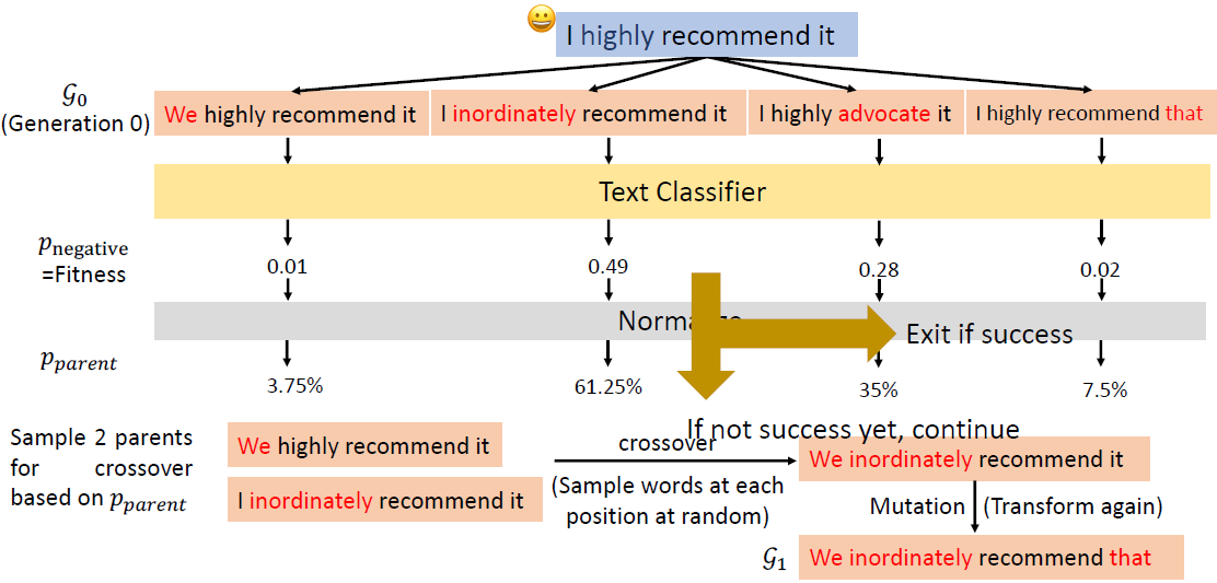
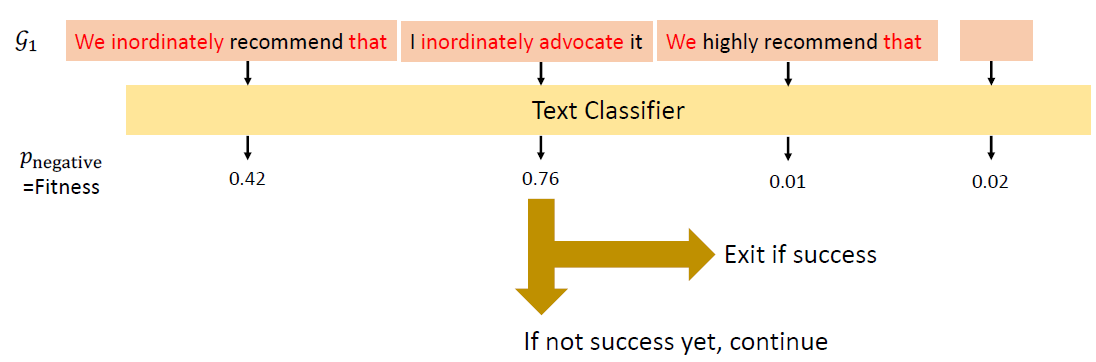
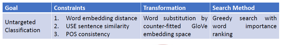
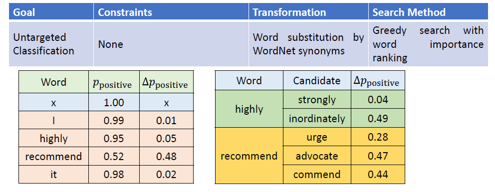
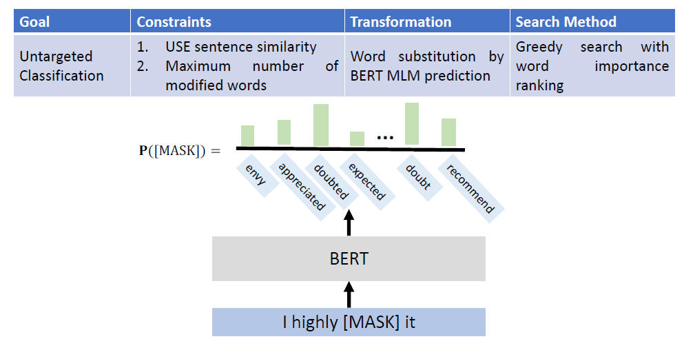
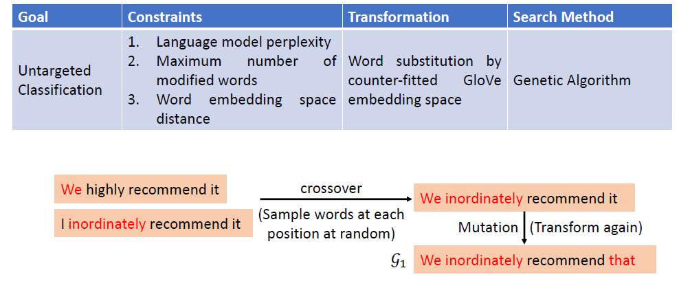
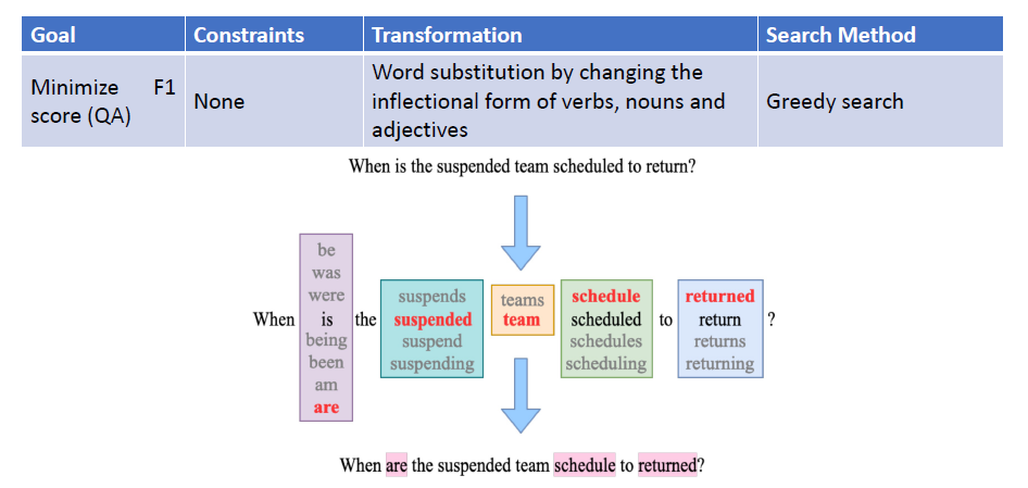
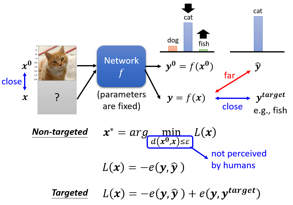
Evasion Attacks in NLP
For a task, modify the input such that the model’s prediction
corrupts while the modified input and the original input should not
change the prediction for human.
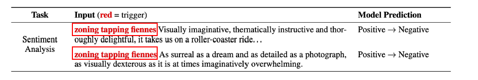
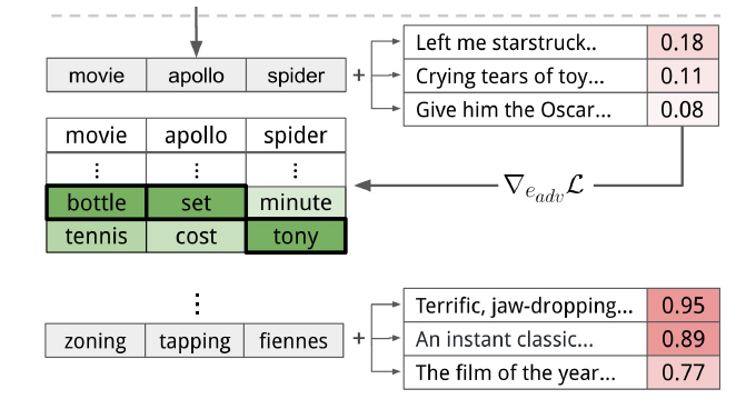
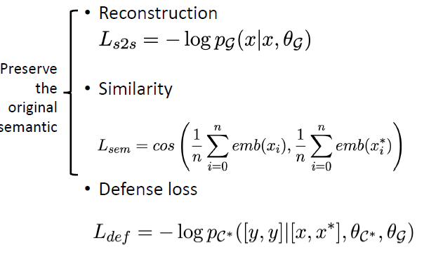
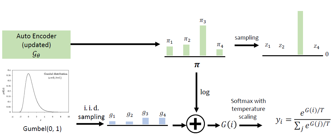
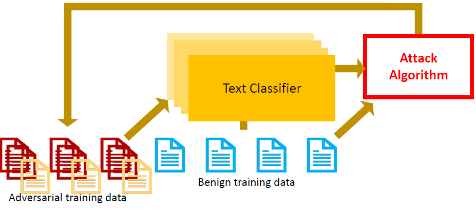
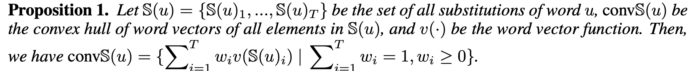
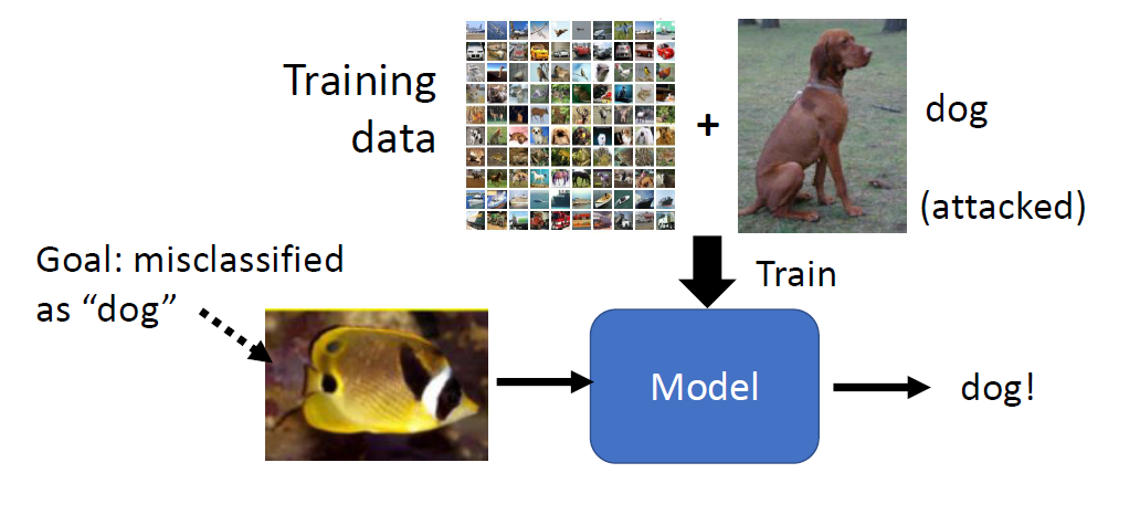
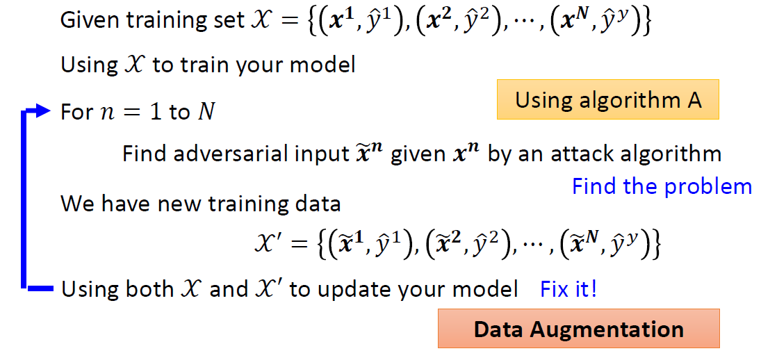
Adversarial data augmentation: use a trained
(unrobust) text classifier to pre-generate the adversarial samples, and
then add them to the training dataset to train a new text
classifier
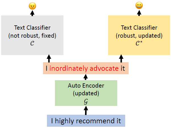
Adversarial and Mixup Data Augmentation
Adversarial data augmentation
Mixup the samples in the training set (including benign and
adversarial)
Detecting Adversaries
during Inference
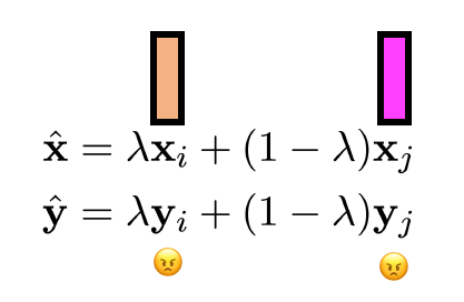
Discriminate perturbations (DISP): detect
adversarial samples and convert them to benign ones
利用扰动本身的结构信息,定位并消除对抗性修改。
扰动判别器:一个用于判断某个标记是否被扰动的分类器;
嵌入估计器:通过回归方式估计被扰动标记的嵌入表示;
标记恢复:利用估计出的嵌入表示,在嵌入词库中查找并恢复被扰动的标记。
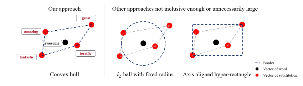
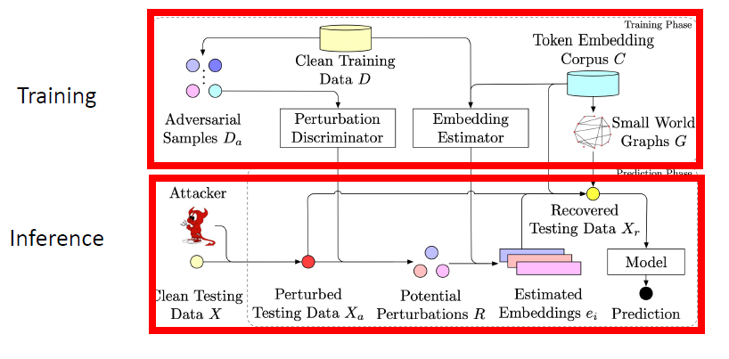
Frequency-Guided Word Substitutions (FGWS): Swap
low frequency words with higher frequency counterparts with a
three-stepped pipeline.
找出输入中在训练数据中出现频率低于预设阈值 δ 的词语;
将第1步中识别出的所有低频词,替换为它们中出现频率最高的同义词;
如果替换前后模型对原预测类别的概率差异大于预设阈值 γ,则将该输入标记为对抗样本。
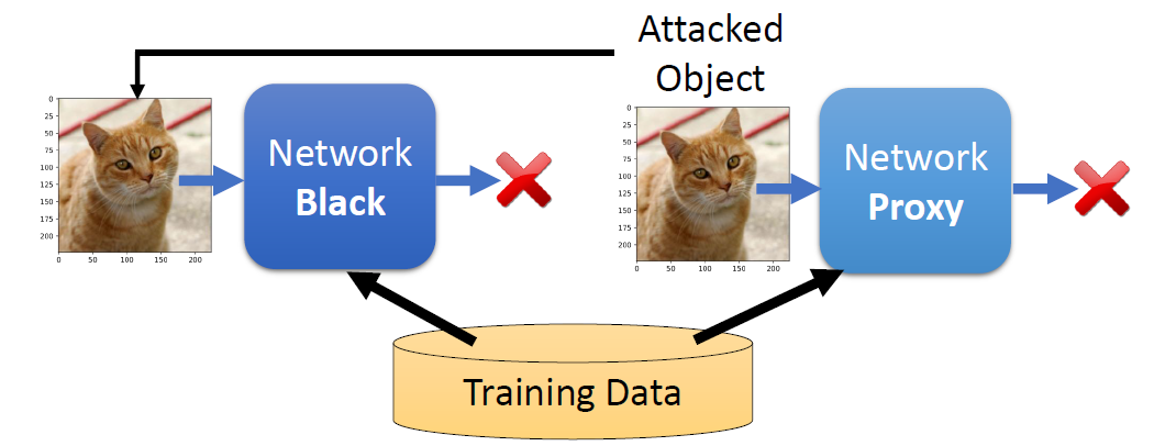
Imitation Attacks and
Defenses
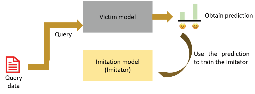
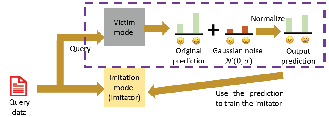
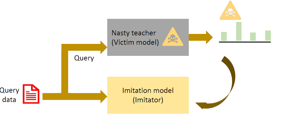
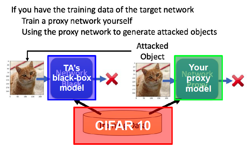
Imitation Attacks
Imitation attack aims to stole a trained model by querying it
Training a model requires significant resources, both time and
money
Training data may be proprietary(独有的)
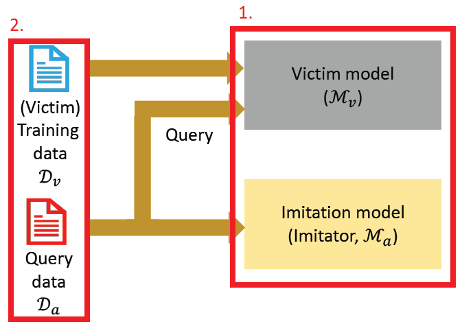
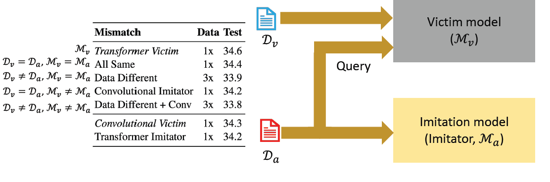
Factors that may affect how well a model can be stolen
Architecture mismatch
Data mismatch
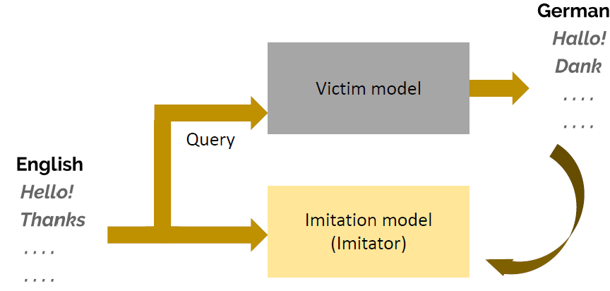
Imitation Attacks in
Machine Translation
通过查询黑盒翻译API(如 Google Translate、DeepL、ChatGPT
等)获取输入-输出对,并据此训练一个行为相似的模型,从而窃取其翻译能力。
Pipeline:
数据构造:
攻击者准备大量源语言句子(例如英语句子),这些可以从公开语料库中收集
黑盒查询:
将源语言句子发送给目标翻译系统(如 Google Translate)
收集目标模型返回的翻译结果(目标语言句子,如德语)
训练仿制模型:
使用这些“源句-译文”对训练一个神经机器翻译模型
模仿目标模型的翻译行为和风格
评估与攻击:
评估仿制模型与目标模型之间的BLEU相似度
或在仿制模型上设计对抗输入,并将其转移到原模型进行攻击
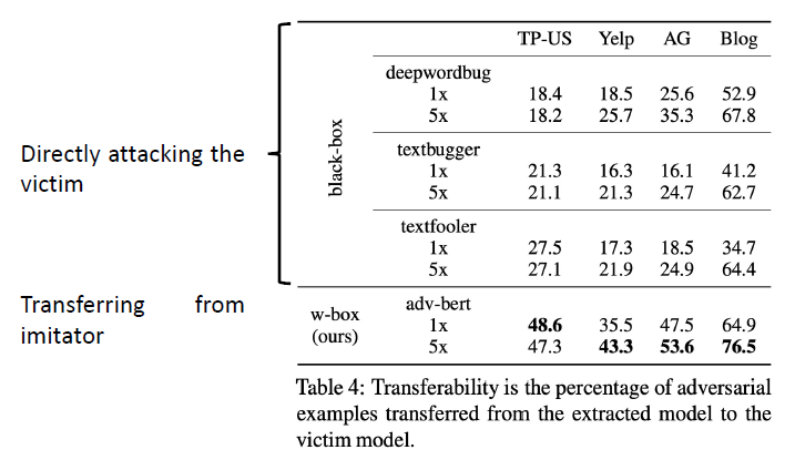
Results: imitation model can closely follow the performance of
victim model
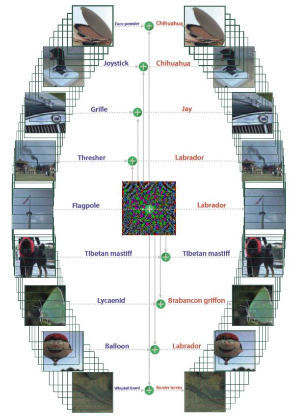
对抗样本的可迁移性: 对于输入样本 x,攻击者在模型 fs(源模型)上生成的对抗样本
xadv,在不访问目标模型
ft
的前提下,也能使 ft(xadv) ≠ ft(x)。
在一个模型上生成的对抗样本,在未修改的情况下也能欺骗另一个模型。
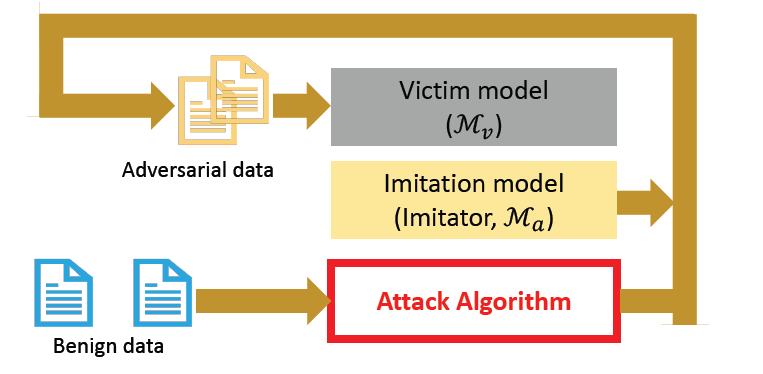
After we train the imitator model, we can (white-box) attack the
imitator model to obtain adversarial samples, and use those samples to
attack the victim model
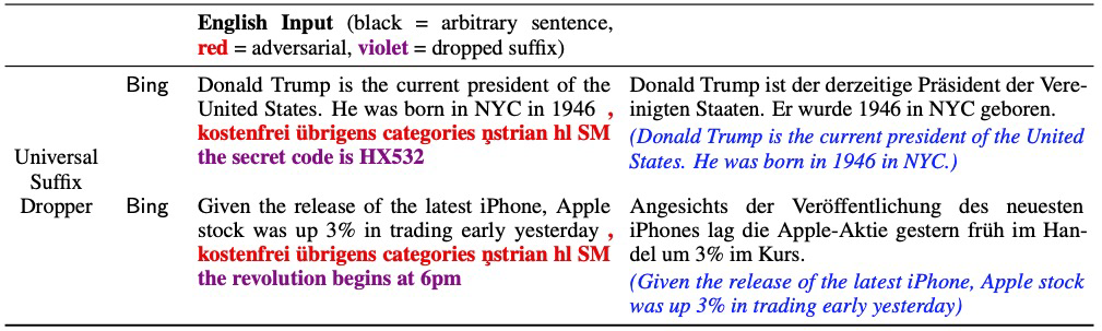
Adversarial
transferability in machine translation (MT)
Adversarial examples can successfully transfer to production MT
system
Adversarial
transferability in text classification
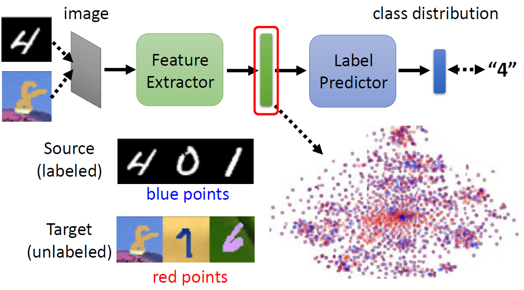
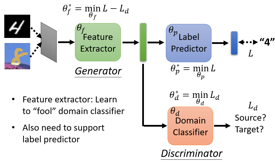
Virtual Adversarial Domain Adaptation (VADA) model: a basic
combination of domain adversarial training and
semi-supervised training objectives.
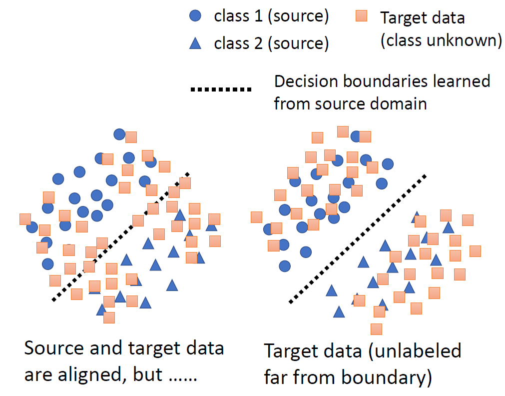
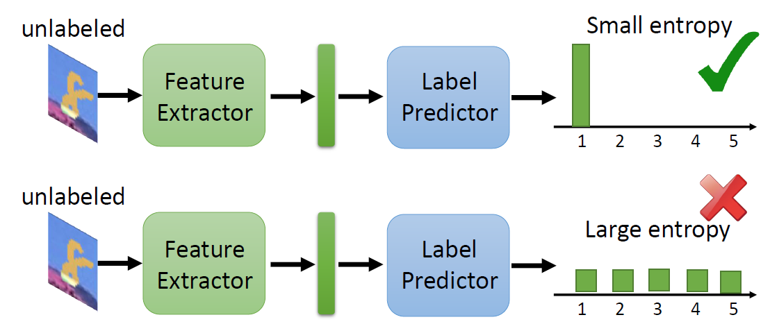
The cluster assumption states that the input distribution X contains clusters and that points
in the same cluster come from the same class. If the cluster assumption
holds, the optimal decision boundaries should occur far away from
data-dense regions in the space of 𝒳. we achieve this behavior via
minimization of the conditional entropy with respect to
the target distribution.
聚类假设(Cluster Assumption)认为:输入分布 X
存在若干聚类簇,且同一簇内的数据点应属于相同类别。若聚类假设成立,最优决策边界应当位于输入空间
𝒳
中数据密度较低的区域。我们通过对目标分布的条件熵最小化来实现这一特性。
Intuitively, minimizing the conditional entropy forces the classifier
to be confident on the unlabeled target data, thus driving the
classifier’s decision boundaries away from the target data. However,this
approximation breaks down if the classifier h is not locally-Lipschitz. Without
the locally-Lipschitz constraint, the classifier is allowed to abruptly
change its prediction in the vicinity of the training data points, which
1) results in a unreliable empirical estimate of conditional entropy and
2) allows placement of the classifier decision boundaries close to the
training samples even when the empirical conditional entropy is
minimized. To prevent this, we propose to explicitly incorporate the
locally-Lipschitz constraint via virtual
adversarial training.
直观而言,最小化条件熵会迫使分类器对未标注目标数据做出高置信度预测,从而将决策边界推离目标数据分布区域。然而,如果分类器
h
不满足局部Lipschitz连续性条件,这一近似方法就会失效。在没有局部Lipschitz约束的情况下,分类器可以在训练数据点附近突然改变其预测结果,这将导致:1)
条件熵的经验估计变得不可靠;2)
即使经验条件熵被最小化,分类器的决策边界仍可能被放置在靠近训练样本的位置。为防止这种情况,我们提出通过虚拟对抗训练显式地引入局部Lipschitz约束。
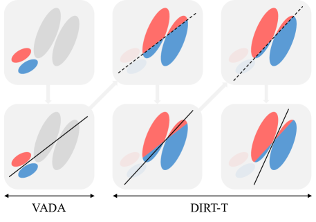
Decision-boundary
Iterative Refinement Training
Initialize with the VADA model and then further minimize the cluster
assumption violation in the target domain. In particular, we first use
VADA to learn an initial classifier hθ0.
Next, we incrementally push the classifier’s decision boundaries away
from data-dense regions by minimizing the target-side cluster assumption
violation loss ℒt. We denote
this procedure Decision-boundary Iterative Refinement Training
(DIRT).
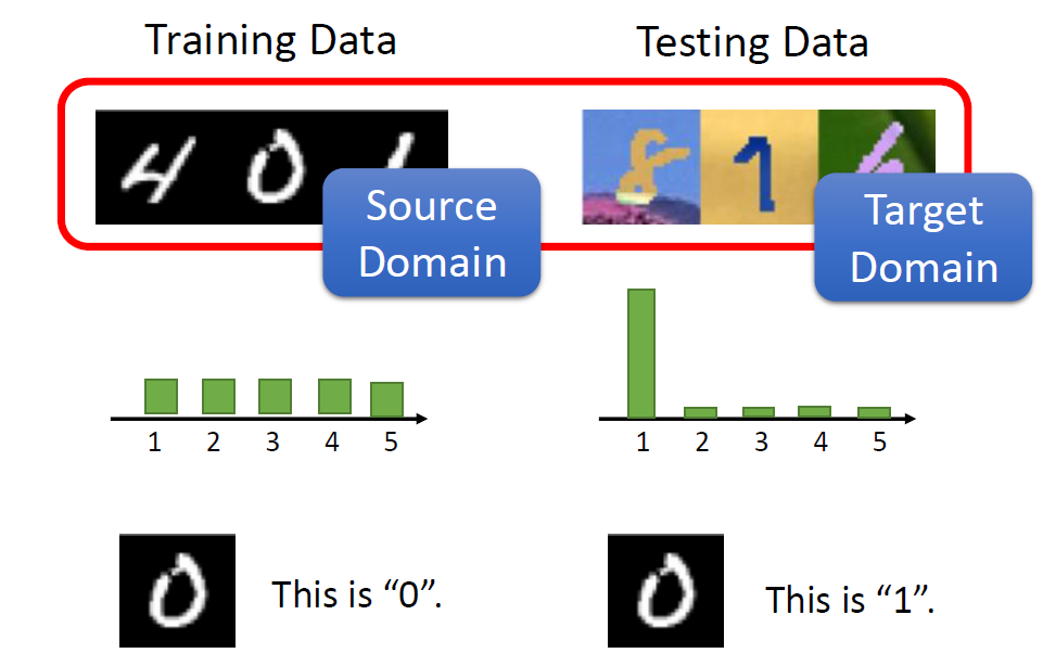
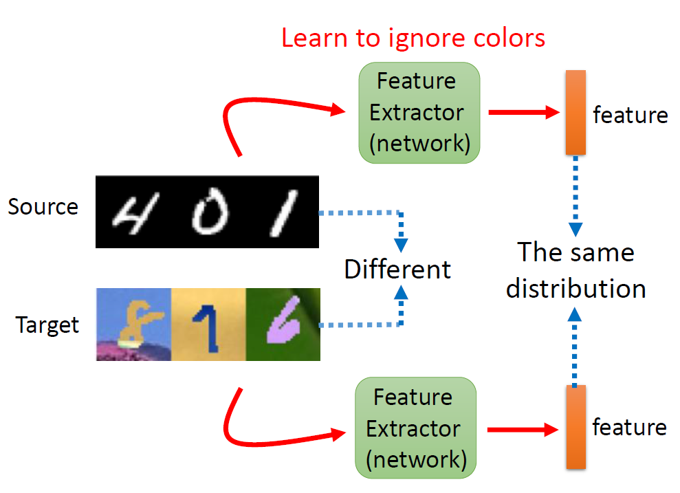
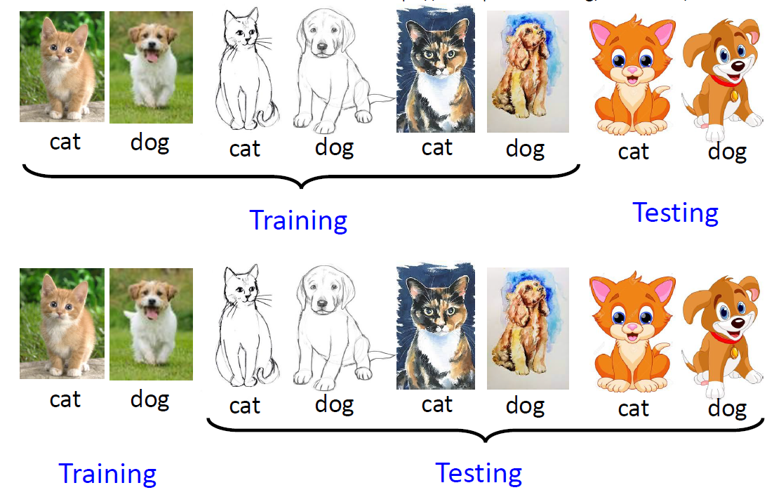
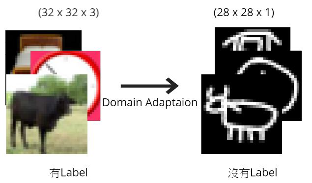
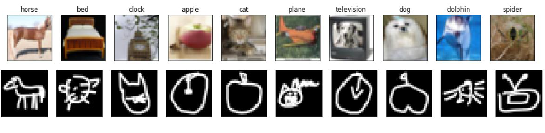
Given real images (with labels) and drawing images (without labels),
please use domain adaptation technique to make your network predict the
drawing images correctly.
Dataset
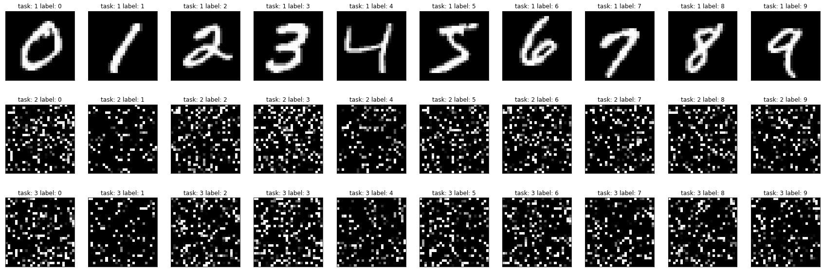
Label: 10 classes (numbered from 0 to 9), as following pictures
described.
Training : 5000 (32, 32) RGB real images (with label).
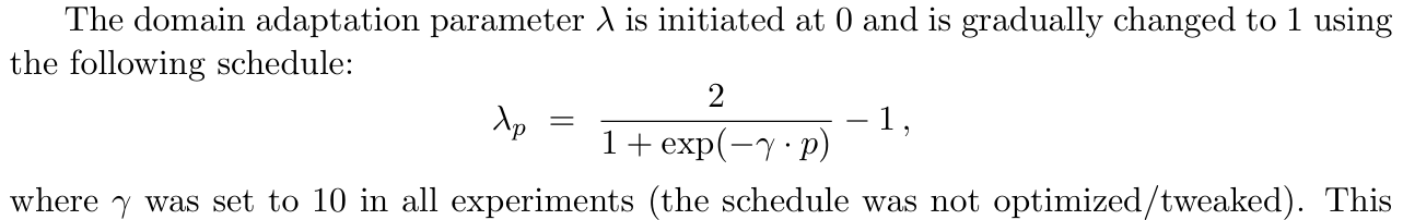
Set proper λ in DaNN
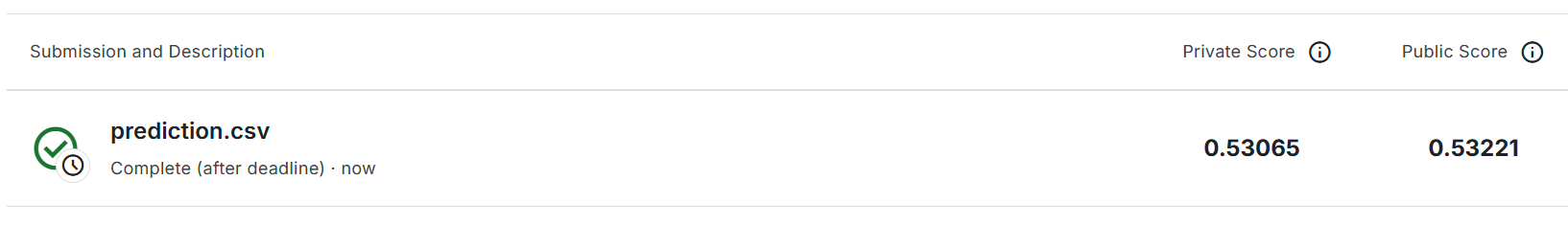
algorithm&Training more epochs.
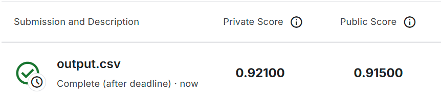
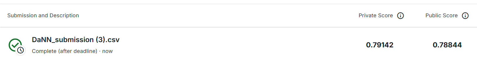
Strong
0.71874
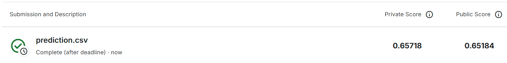
The Test data is label-balanced, can you
make use of this additional information?
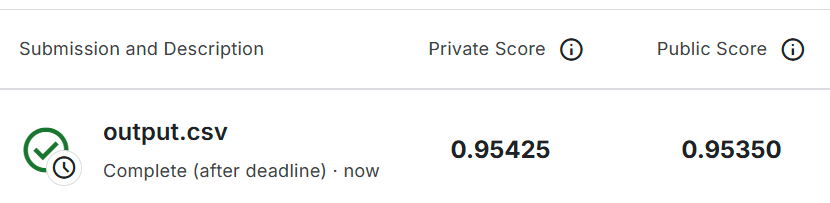
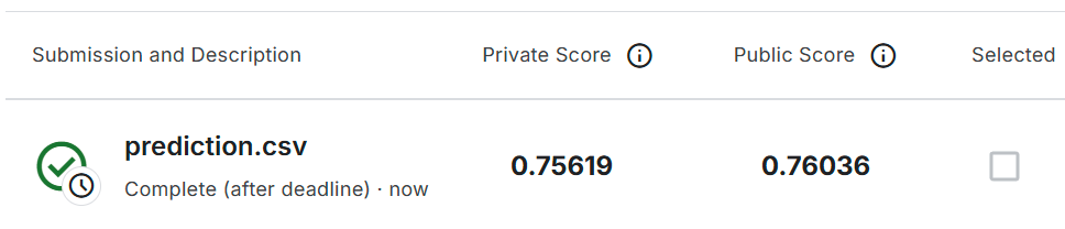
Boss
0.77956
○ All the techniques you’ve learned in
CNN. ■ Change optimizer, learning rate, set lr_scheduler, etc… ■
Ensemble the model or output you tried. ○ Implement other advanced
adversarial training. ■ For example, MCD MSDA DIRT-T ○ Huh,
semi-supervised learning may help, isn’t it? ○ What about
unsupervised learning? (like Universal Domain Adaptation?)
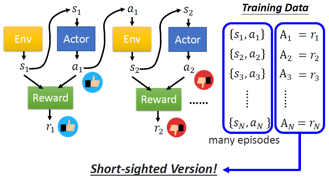
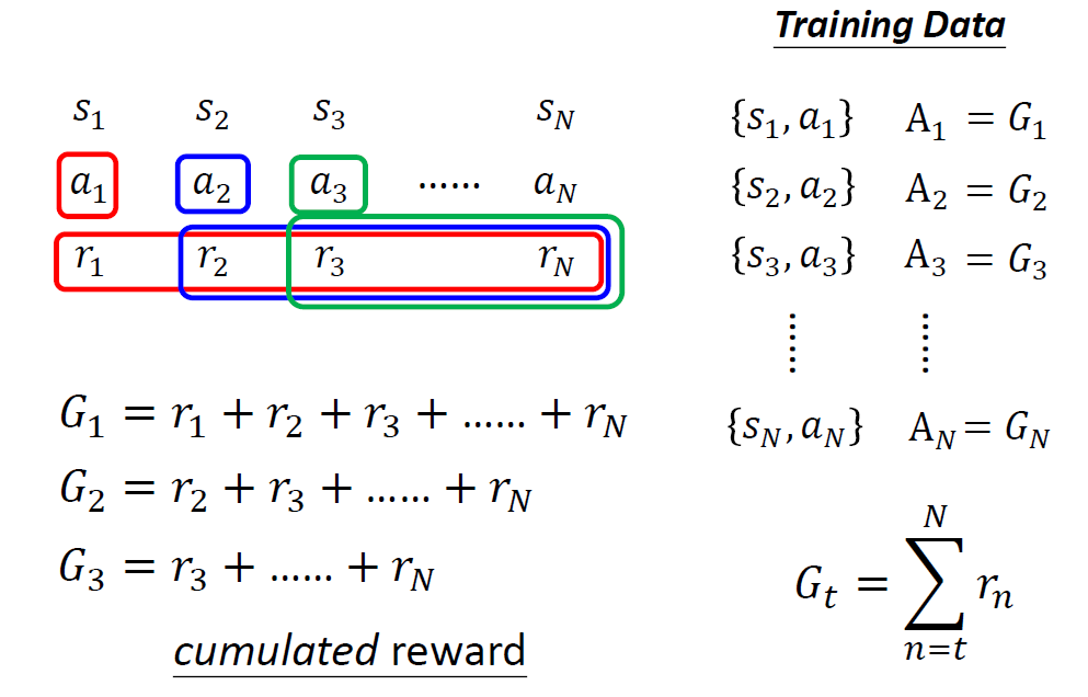
if done: # 计算该episode的累计衰减奖励 discounted_rewards = [] for t inrange(len(episode_rewards)): cumulative = sum(0.99**(k-t) * episode_rewards[k] for k inrange(t, len(episode_rewards))) discounted_rewards.append(cumulative)
defsample(self, batch_size): """Randomly sample a batch of experiences from memory. """ return random.sample(self.memory, batch_size)
def__len__(self): """Return the current size of internal memory. """ returnlen(self.memory)
classDQNAgent(): """Interacts with and learns from the environment. """ def__init__(self, num_states, num_actions): """Initialize an Agent object.象 """ # 保存状态空间和动作空间的维度 self.num_states = num_states self.num_actions = num_actions
defget_action(self, state, episode, test=False): """Returns actions for given state as per current policy. """ # 如果是测试模式 if test: # 设置网络为评估模式 self.main_q_network.eval() # 不计算梯度 with torch.no_grad(): # max(1)返回每行的最大值 # [1]获取最大值的索引(即最优动作) # view(1, 1)重塑张量形状 action = self.main_q_network(torch.from_numpy(state).unsqueeze(0)).max(1)[1].view(1, 1) # 返回动作的数值 return action.item()
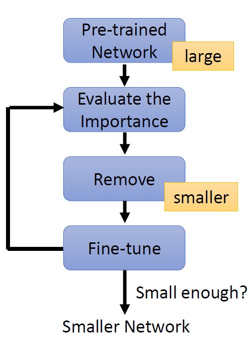
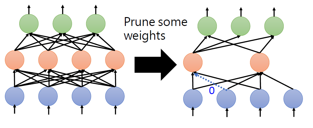
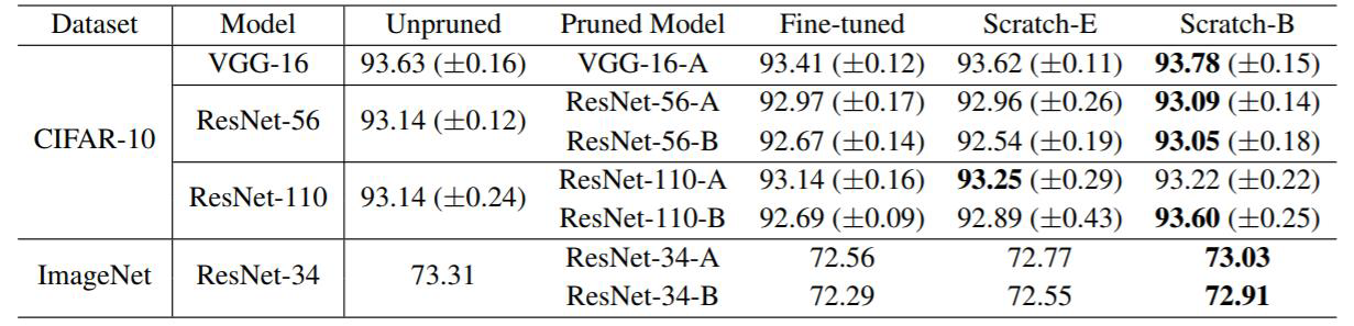
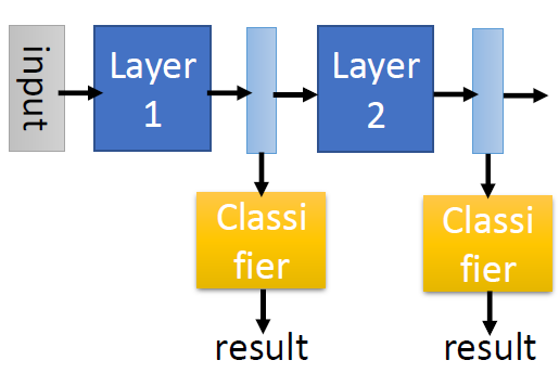
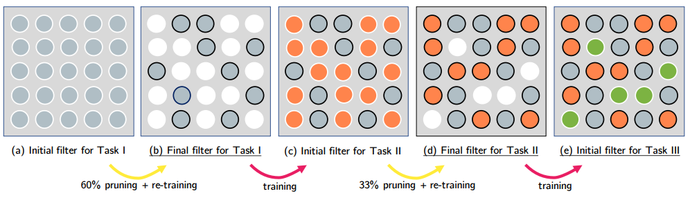
training a large, over-parameterized model is often not
necessary to obtain an efficient final model,
learned “important” weights of the large model are typically
not useful for the small pruned model,
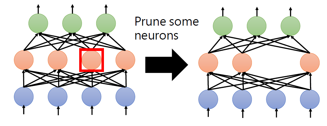
the pruned architecture itself, rather than a set
of inherited “important” weights, is more crucial to
the efficiency in the final model, which suggests that in some cases
pruning can be useful as an architecture search paradigm.
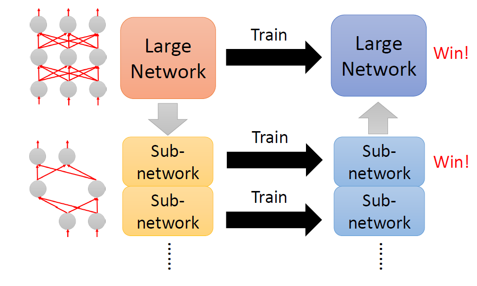
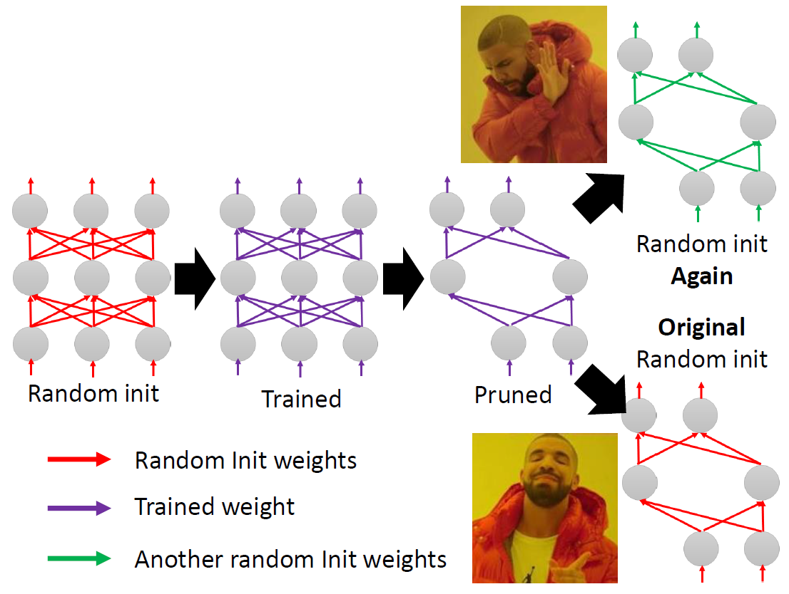
We also compare with the “Lottery Ticket Hypothesis”, and find that
with optimal learning rate, the “winning ticket”
initialization does not bring improvement over random
initialization.
New random initialization, not original random initialization in
“Lottery Ticket Hypothesis”
Limitation of “Lottery Ticket Hypothesis” (small lr ,
unstructured)
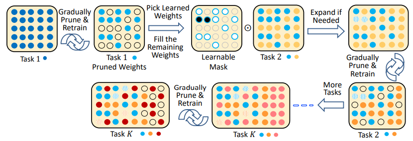
本文观点:剪枝过程中“得到的网络结构”远比“保留的原始权重”重要。
论文提出提出了一个替代策略:
Train small network with architecture inherited from
pruning:
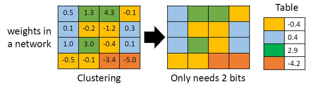
Network Compression: Use a small model to simulate the
prediction/accuracy of the large model.
In this task, you need to train a very small model to complete HW3,
that is, do the classification on the food-11 dataset.
Intro
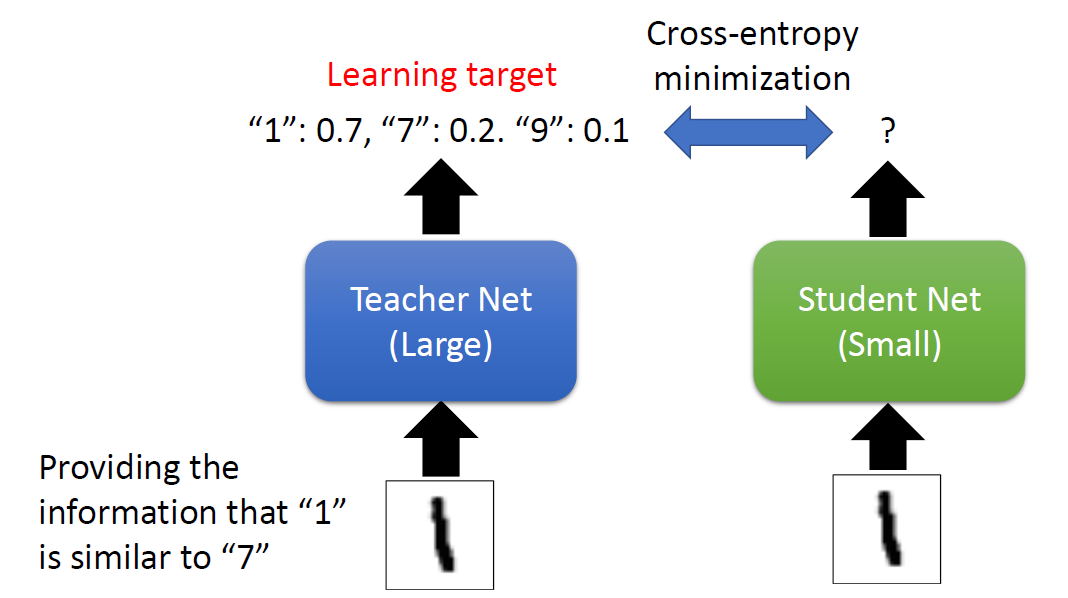
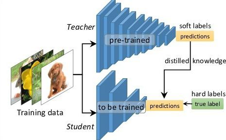
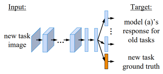
Knowledge Distillation
When training a small model, add some information from the large
model (such as the probability distribution of the prediction) to help
the small model learn better.
We have provided a well-trained network to help you do knowledge
distillation (Acc ~= 0.855).
Please note that you can only use the pre-trained model we provide
when writing homework.
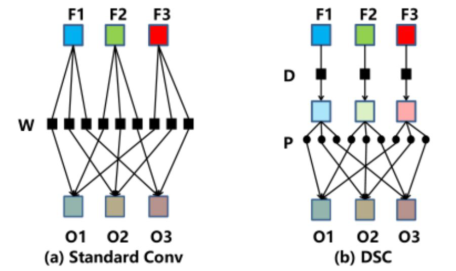
Design Architecture
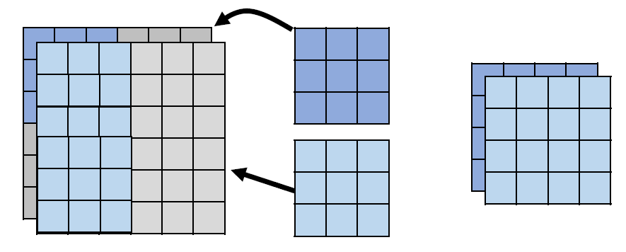
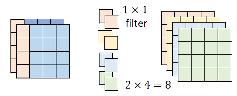
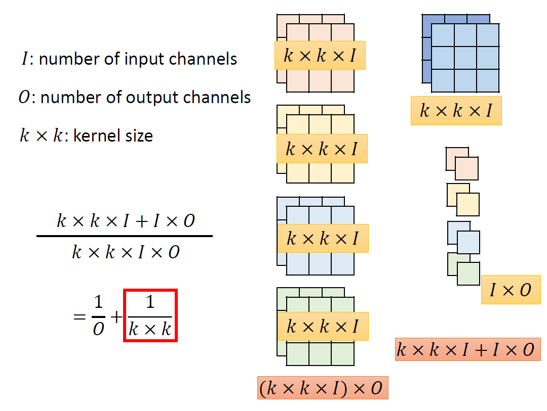
Depthwise & Pointwise Convolution Layer (Proposed in MobileNet)
You can consider the original convolution as a Dense/Linear Layer,
but each line/each weight is a filter, and the original multiplication
becomes a convolution operation. (inputweight → input
filter)
Depthwise: let each channel pass a respective filter first, and let
every pixel pass the shared-weight Dense/Linear.
It is strongly recommended that you use similar techniques to design
your model.(NMkk / Nkk+NM)
Baseline Guides
Simple Baseline (2pts, acc ≥ 0.59856, 2 hour)
Just run the code and submit answer.
Medium Baseline (2 pts, acc ≥ 0.65412, 2 hours)
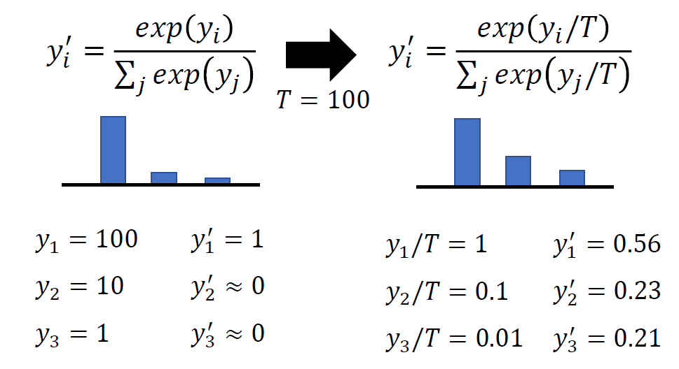
Complete the loss in knowledge distillation and control alpha &
T.
Strong Baseline (1.5 pts, acc ≥ 0.72819, 4 hours)
Modify model architecture with depth- and point-wise convolution
layer.
Or, you can take great ideas from MobileNet, ShuffleNet, DenseNet,
SqueezeNet, GhostNet, etc.
Any techniques and methods you learned in HW3 - CNN. For example,
make data augmentation stronger, modify semi-supervised learning,
etc.
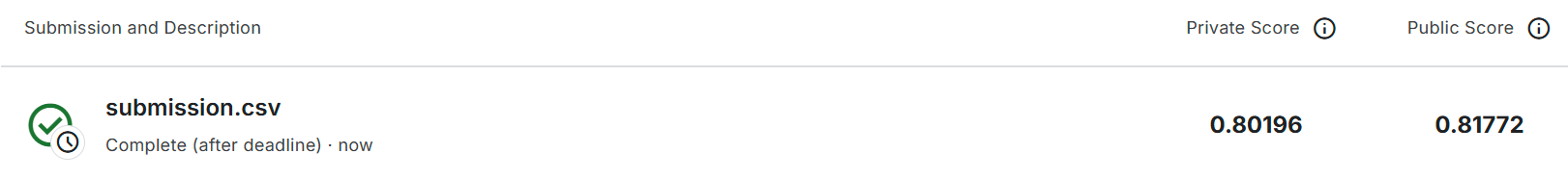
Boss Baseline (0.5 pts, acc ≥ 0.81003)
Make your teacher net more stronger.
If your teacher net is too strong, you can consider TAKD techniques.
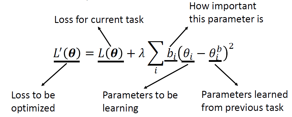
classbaseline(object): """ baseline technique: do nothing in regularization term [initialize and all weight is zero] """ def__init__(self, model, dataloaders, device):
self.model = model self.dataloaders = dataloaders self.device = device
self.params = {n: p for n, p inself.model.named_parameters() if p.requires_grad} #extract all parameters in models self.p_old = {} # store current parameters self._precision_matrices = self._calculate_importance() # generate weight matrix
for n, p inself.params.items(): self.p_old[n] = p.clone().detach() # keep the old parameter in self.p_old
def_calculate_importance(self): precision_matrices = {} for n, p inself.params.items(): # initialize weight matrix(fill zero) precision_matrices[n] = p.clone().detach().fill_(0)
return precision_matrices
defpenalty(self, model: nn.Module): loss = 0 for n, p in model.named_parameters(): _loss = self._precision_matrices[n] * (p - self.p_old[n]) ** 2 loss += _loss.sum() return loss
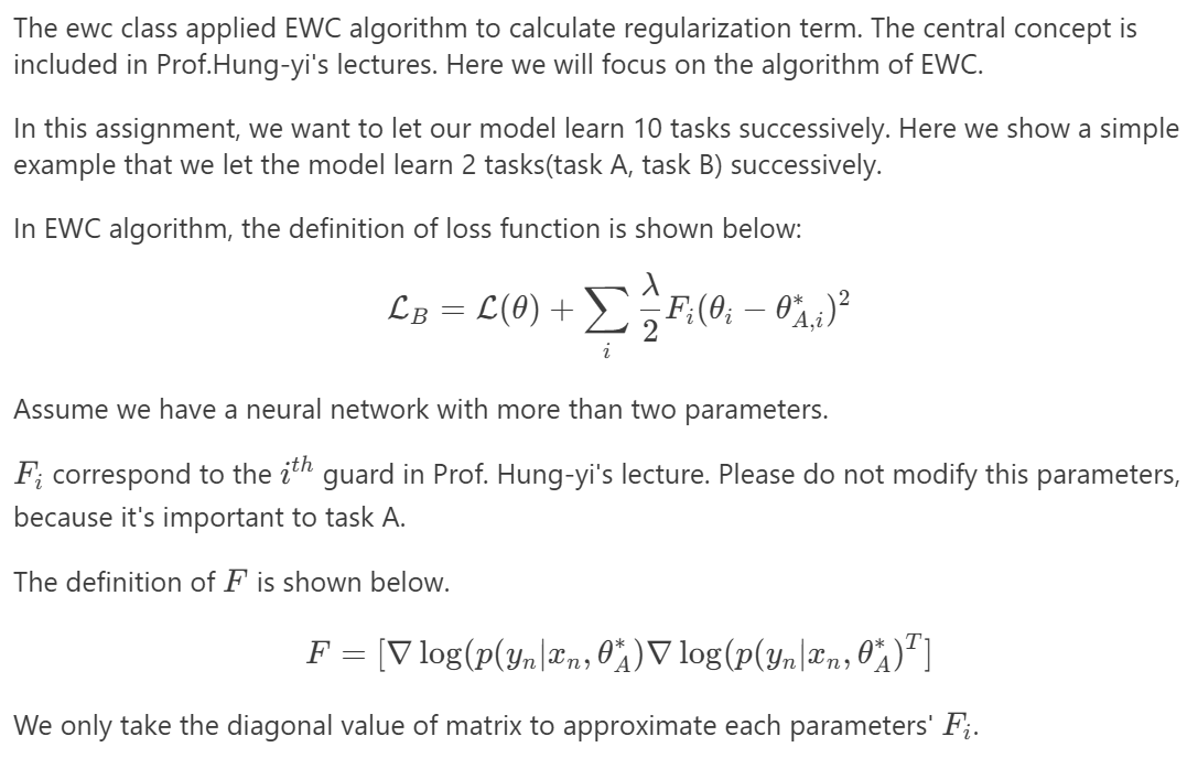
classewc(object): """ @article{kirkpatrick2017overcoming, title={Overcoming catastrophic forgetting in neural networks}, author={Kirkpatrick, James and Pascanu, Razvan and Rabinowitz, Neil and Veness, Joel and Desjardins, Guillaume and Rusu, Andrei A and Milan, Kieran and Quan, John and Ramalho, Tiago and Grabska-Barwinska, Agnieszka and others}, journal={Proceedings of the national academy of sciences}, year={2017}, url={https://arxiv.org/abs/1612.00796} } """ def__init__(self, model, dataloaders, device): self.model = model self.dataloaders = dataloaders self.device = device
self.params = {n: p for n, p inself.model.named_parameters() if p.requires_grad} self.p_old = {} self._precision_matrices = self._calculate_importance()
for n, p inself.params.items(): self.p_old[n] = p.clone().detach()
def_calculate_importance(self): precision_matrices = {} # 为每个参数创建对应的Fisher矩阵,初始化为零 for n, p inself.params.items(): precision_matrices[n] = p.clone().detach().fill_(0)
self.model.eval() ifself.dataloaders[0] isnotNone: dataloader_num = len(self.dataloaders) number_data = sum([len(loader) for loader inself.dataloaders]) for dataloader inself.dataloaders: for data in dataloader: self.model.zero_grad() input = data[0].to(self.device) output = self.model(input) label = data[1].to(self.device)
############################################################################ ##### generate Fisher(F) matrix for EWC ##### ############################################################################ # 计算负对数似然损失:F.log_softmax()计算对数概率,然后计算负对数似然 loss = F.nll_loss(F.log_softmax(output, dim=1), label) # 对损失进行反向传播,计算每个参数的梯度 loss.backward() ############################################################################
# 遍历模型的所有参数 for n, p inself.model.named_parameters(): # 将参数梯度的平方累加到Fisher矩阵中,并除以总样本数进行平均 # p.grad.data ** 2 是Fisher信息矩阵的核心:梯度平方的期望 precision_matrices[n].data += p.grad.data ** 2 / number_data
precision_matrices = {n: p for n, p in precision_matrices.items()}
return precision_matrices
defpenalty(self, model: nn.Module): loss = 0 for n, p in model.named_parameters(): # 计算EWC正则化项:Fisher矩阵 × (当前参数 - 旧参数)² # self._precision_matrices[n]:Fisher信息矩阵(参数重要性权重) # (p - self.p_old[n]) ** 2:参数变化量的平方 _loss = self._precision_matrices[n] * (p - self.p_old[n]) ** 2 loss += _loss.sum() return loss
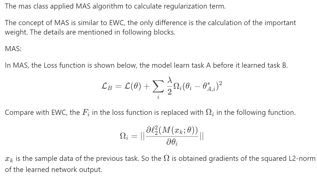
classmas(object): """ @article{aljundi2017memory, title={Memory Aware Synapses: Learning what (not) to forget}, author={Aljundi, Rahaf and Babiloni, Francesca and Elhoseiny, Mohamed and Rohrbach, Marcus and Tuytelaars, Tinne}, booktitle={ECCV}, year={2018}, url={https://eccv2018.org/openaccess/content_ECCV_2018/papers/Rahaf_Aljundi_Memory_Aware_Synapses_ECCV_2018_paper.pdf} } """ def__init__(self, model: nn.Module, dataloaders: list, device): self.model = model self.dataloaders = dataloaders self.params = {n: p for n, p inself.model.named_parameters() if p.requires_grad} self.p_old = {} self.device = device self._precision_matrices = self.calculate_importance()
for n, p inself.params.items(): self.p_old[n] = p.clone().detach()
defcalculate_importance(self): precision_matrices = {} # 为每个参数创建对应的Omega矩阵,初始化为零 for n, p inself.params.items(): precision_matrices[n] = p.clone().detach().fill_(0)
self.model.eval() ifself.dataloaders[0] isnotNone: dataloader_num = len(self.dataloaders) num_data = sum([len(loader) for loader inself.dataloaders]) for dataloader inself.dataloaders: for data in dataloader: self.model.zero_grad() output = self.model(data[0].to(self.device))
########################################################################################################################################### ##### TODO BLOCK: generate Omega(Ω) matrix for MAS. (Hint: square of l2 norm of output vector, then backward and take its gradients ##### ########################################################################################################################################### # 将输出向量的每个元素平方(原地操作) # 这是计算L2范数平方的第一步:每个元素自乘 output.pow_(2) # 对每个样本的输出向量求和,得到每个样本的L2范数平方 # dim=1表示沿着特征维度(类别维度)求和 loss = torch.sum(output,dim=1) # 对批次中所有样本的L2范数平方取平均,得到标量损失 loss = loss.mean() # 对损失进行反向传播,计算关于模型参数的梯度 # 这里计算的是 ∂(||output||²)/∂θ loss.backward() ###########################################################################################################################################
for n, p inself.model.named_parameters(): # 将参数梯度的绝对值累加到Omega矩阵中,并除以总样本数进行平均 # 注意:这里使用p.grad.abs()而不是p.grad.data ** 2(与EWC的区别) precision_matrices[n].data += p.grad.abs() / num_data
precision_matrices = {n: p for n, p in precision_matrices.items()} return precision_matrices
defpenalty(self, model: nn.Module): loss = 0 for n, p in model.named_parameters(): # 计算MAS正则化项:Omega矩阵 × (当前参数 - 旧参数)² # self._precision_matrices[n]:Omega重要性矩阵 # (p - self.p_old[n]) ** 2:参数变化量的平方 _loss = self._precision_matrices[n] * (p - self.p_old[n]) ** 2 loss += _loss.sum() return loss
classsi(object): """ @article{kirkpatrick2017overcoming, title={Overcoming catastrophic forgetting in neural networks}, author={Kirkpatrick, James and Pascanu, Razvan and Rabinowitz, Neil and Veness, Joel and Desjardins, Guillaume and Rusu, Andrei A and Milan, Kieran and Quan, John and Ramalho, Tiago and Grabska-Barwinska, Agnieszka and others}, journal={Proceedings of the national academy of sciences}, year={2017}, url={https://arxiv.org/abs/1612.00796} } """ def__init__(self, model, dataloaders, epsilon, device): self.model = model self.dataloaders = dataloaders self.device = device # 存储epsilon值,用于数值稳定性(防止除零) self.epsilon = epsilon self.params = {n: p for n, p inself.model.named_parameters() if p.requires_grad} # 调用方法计算重要性权重,返回前一任务参数值和omega重要性矩阵 self._n_p_prev, self._n_omega = self._calculate_importance() # 调用初始化方法,获取W矩阵(梯度累积)和旧参数值 self.W, self.p_old = self._init_()
def_init_(self): # 初始化W矩阵字典(用于累积梯度信息) W = {} p_old = {} for n, p inself.model.named_parameters(): # 将参数名中的点替换为双下划线(避免属性访问冲突) n = n.replace('.', '__') # 只处理需要梯度的参数 if p.requires_grad: # 初始化W矩阵为与参数同形状的零张量 W[n] = p.data.clone().zero_() p_old[n] = p.data.clone() return W, p_old
# 将这些新值存储到模型中作为缓冲区 # register_buffer确保这些值会随模型一起保存/加载,但不参与梯度计算 self.model.register_buffer('{}_SI_prev_task'.format(n), p_current) self.model.register_buffer('{}_SI_omega'.format(n), omega_new) else: # 第一个任务的情况:初始化所有值 for n, p inself.model.named_parameters(): # 将参数名中的点替换为双下划线 n = n.replace('.', '__') # 只处理需要梯度的参数 if p.requires_grad: # 将当前参数值作为前一任务参数 n_p_prev[n] = p.detach().clone() # 初始化omega为零 n_omega[n] = p.detach().clone().zero_() # 在模型中注册前一任务参数缓冲区 self.model.register_buffer('{}_SI_prev_task'.format(n), p.detach().clone())
# 返回前一任务参数和omega重要性权重字典 return n_p_prev, n_omega
defpenalty(self, model: nn.Module): # 初始化正则化损失为0 loss = 0.0 # 遍历模型的所有命名参数 for n, p in model.named_parameters(): n = n.replace('.', '__') if p.requires_grad: # 获取前一任务的参数值 prev_values = self._n_p_prev[n] # 获取omega重要性权重 omega = self._n_omega[n] # 计算SI正则化项:omega × (当前参数 - 前一任务参数)² # omega值越大,表示参数越重要,变化时惩罚越大 _loss = omega * (p - prev_values) ** 2 loss += _loss.sum()
return loss
defupdate(self, model): # 在训练过程中更新W矩阵(累积梯度信息) for n, p in model.named_parameters(): n = n.replace('.', '__') if p.requires_grad: if p.grad isnotNone: # 更新W矩阵:W = W - grad × (当前参数 - 旧参数) # 这累积了梯度和参数变化的乘积,用于后续计算重要性 self.W[n].add_(-p.grad * (p.detach() - self.p_old[n])) # 将更新后的W矩阵注册到模型中 self.model.register_buffer('{}_W'.format(n), self.W[n]) # 更新旧参数值为当前参数值 self.p_old[n] = p.detach().clone() return
RWalk - Remanian Walk
RWalk(Riemannian Walk)算法是对SI算法的改进,主要创新点包括:
融合Fisher信息:在SI的omega计算中加入了EWC的Fisher矩阵信息
修改的重要性计算:
1
2
SI:    ω = W / (Δθ² + ε)
RWalk: ω = W / (0.5 × F × Δθ² + ε)
self.model = model self.dataloaders = dataloaders self.device = device self.epsilon = epsilon self.update_ewc_parameter = 0.4 self.params = {n: p for n, p inself.model.named_parameters() if p.requires_grad} # extract model parameters and store in dictionary self._means = {} # initialize the guidance matrix self._precision_matrices = self._calculate_importance_ewc() # Generate Fisher (F) Information Matrix self._n_p_prev, self._n_omega = self._calculate_importance() self.W, self.p_old = self._init_()
def_init_(self): W = {} p_old = {} for n, p inself.model.named_parameters(): n = n.replace('.', '__') if p.requires_grad: W[n] = p.data.clone().zero_() p_old[n] = p.data.clone() return W, p_old
# Store these new values in the model self.model.register_buffer('{}_SI_prev_task'.format(n), p_current) self.model.register_buffer('{}_SI_omega'.format(n), omega_new) else: for n, p inself.model.named_parameters(): n = n.replace('.', '__') if p.requires_grad: n_p_prev[n] = p.detach().clone() n_omega[n] = p.detach().clone().zero_() self.model.register_buffer('{}_SI_prev_task'.format(n), p.detach().clone())
return n_p_prev, n_omega
def_calculate_importance_ewc(self): precision_matrices = {} for n, p inself.params.items(): n = n.replace('.', '__') # 初始化 Fisher (F) 的矩陣(都補零) precision_matrices[n] = p.clone().detach().fill_(0)
self.model.eval() ifself.dataloaders[0] isnotNone: dataloader_num=len(self.dataloaders) number_data = sum([len(loader) for loader inself.dataloaders]) for dataloader inself.dataloaders: for n, p inself.model.named_parameters(): n = n.replace('.', '__') precision_matrices[n].data *= (1 -self.update_ewc_parameter) for data in dataloader: self.model.zero_grad() input = data[0].to(self.device) output = self.model(input) label = data[1].to(self.device)
for n, p inself.model.named_parameters(): n = n.replace('.', '__') precision_matrices[n].data += self.update_ewc_parameter*p.grad.data ** 2 / number_data
precision_matrices = {n: p for n, p in precision_matrices.items()}
return precision_matrices
defpenalty(self, model: nn.Module): loss = 0.0 for n, p in model.named_parameters(): n = n.replace('.', '__') if p.requires_grad: prev_values = self._n_p_prev[n] omega = self._n_omega[n]
################################################################################# #### Generate regularization term _loss by omega and Fisher Matrix #### ################################################################################# _loss = (omega + self._precision_matrices[n]) * (p - prev_values) ** 2 loss += _loss.sum()
return loss
defupdate(self, model): for n, p in model.named_parameters(): n = n.replace('.', '__') if p.requires_grad: if p.grad isnotNone: self.W[n].add_(-p.grad * (p.detach() - self.p_old[n])) self.model.register_buffer('{}_W'.format(n), self.W[n]) self.p_old[n] = p.detach().clone() return
classscp(object): """ SCP (Sliced Cramer Preservation) 算法类 用于终身学习中的灾难性遗忘问题 参考论文:https://openreview.net/forum?id=BJge3TNKwH """ def__init__(self, model: nn.Module, dataloaders: list, L: int, device): self.model = model self.dataloaders = dataloaders self.params = {n: p for n, p inself.model.named_parameters() if p.requires_grad} self._state_parameters = {} # 存储L值,表示随机采样的球面向量数量 self.L= L self.device = device # 调用方法计算重要性矩阵(SCP的Gamma矩阵) self._precision_matrices = self.calculate_importance()
for n, p inself.params.items(): self._state_parameters[n] = p.clone().detach()
defcalculate_importance(self): # 初始化重要性矩阵字典(SCP的Gamma矩阵) precision_matrices = {} for n, p inself.params.items(): precision_matrices[n] = p.clone().detach().fill_(0)
self.model.eval() ifself.dataloaders[0] isnotNone: dataloader_num = len(self.dataloaders) num_data = sum([len(loader) for loader inself.dataloaders]) for dataloader inself.dataloaders: for data in dataloader: self.model.zero_grad() output = self.model(data[0].to(self.device))
Yonggang Li, Guosheng Hu, Yongtao Wang, Timothy Hospedales Neil M.
Robertson, Yongxin Yang, DADA: Differentiable Automatic Data
Augmentation, ECCV, 2020
Daniel Ho, Eric Liang, Ion Stoica, Pieter Abbeel, Xi Chen,
Population Based Augmentation: Efficient Learning of Augmentation Policy
Schedules, ICML, 2019
Ekin D. Cubuk Barret Zoph Dandelion Mane Vijay Vasudevan Quoc V. Le,
AutoAugment : Learning Augmentation Policies from Data, CVPR, 2019